


-
中国林业发展态势良好。以浙江省为例, 2015年林业产业总产值为4 522.87亿元, 比2001年增长3 869.15亿元, 年均增幅达42.28%。与此同时, 森林资源也在逐年增长, 2015年森林蓄积2.97亿m3, 比2001年增长1.59亿m3, 年均涨幅8.22%。森林资源是林业产业的基础, 林业产业从森林培育开始, 产业链一直延伸到森林资源的加工利用及森林旅游等各个产业, 两者关系千丝万缕。只有理清森林资源与林业产业的关系, 把握好它们的发展趋势, 才能更好地利用森林资源, 发展林业产业。通过研究森林资源与林业产业的关系, 对促进林业可持续发展, 更好地在“十三五”时期实现“在保护中发展, 在发展中保护”有着重要的意义。
-
国外对林业研究起步较早, 从17世纪德国创立的森林永续利用理论, 到森林多功能效益理论、林业分工论、新林业理论、近自然林业理论、生态林业理论, 直至21世纪的森林可持续经营理论都阐述了森林资源与经济社会状况的关系。国内相关研究相对起步较晚, 石春娜等[1]对森林资源变化与经济增长进行相关性分析, 证明森林资源变化与经济增长相关。王馨迪[2]、沈月琴等[3]、李成茂[4]分别对浙江省森林资源与林业产业现状、相关性和优势度进行了分析, 得出森林资源量增长与林业产值具有一致性的结论。众多学者都认为森林资源与经济发展存在一定关系, 本研究尝试利用环境库兹涅茨曲线(environmental Kuznets curve, EKC)模型研究森林资源与林业产业的关系。1954年, KUZNETS提出库兹涅茨曲线(又称倒“U”型曲线), 认为在经济发展过程中, 由于各种错综复杂的原因, 人民收入差距会先扩大再缩小[5]。1991年, 美国环境经济学家GROSSMAN等[6]首次实证了环境质量和人均收入的关系, 认为一个国家或地区污染在低收入水平上随人均国内生产总值(GDP)增加而上升, 高收入水平上随人均GDP增长而下降。而环境库兹涅茨曲线则由PANAYOTOU[7]正式提出, 认为环境质量和人均收入也呈倒“U”型曲线, 环境污染在低收入水平会随人均收入增加而上升, 在高收入水平会随人均收入增长而下降。但由于城市化水平、产业结构、环保投资等各种因素都可能会产生直接或间接的影响, 导致不同曲线的出现。
环境污染、能源消耗、生态破坏都影响着环境质量, 因此学者开始把资源变化与经济发展的关系是否存在EKC曲线, 逐渐延伸到林业领域, 但主要从宏观经济验证与森林资源的关系。CHEN等[8], AHMED等[9], MBATU[10]分别以中国、巴基斯坦、喀麦隆为研究对象, 以EKC理论研究经济发展与森林资源的关系; 许姝明[11], 李鲁欣[12], 王凯等[13]分别将全国及江西省、山东省的人均GDP为经济指标, 运用EKC模型研究经济增长与森林资源的变化关系。
近年来, 学者将EKC模型应用由宏观经济向各领域经济探索。史磊等[14], 张中华[15]分别以人均农业产值、人均农林牧渔产值作为农业经济的指标, 研究农业经济增长与农业面源的关系。付秀梅等[16]以海洋生产总值作为反映海洋经济的指标, 实证分析了海洋经济增长与环境污染水平关系。赵贺春等[17]以铝工业总产值作为经济指标, 从整体上研究中国铝业发展与其造成环境负荷之间的关系。张锡等[18]选取2000-2013年浙江进出口总值测度外贸发展水平, 构建环境库兹涅茨曲线并分析浙江省对外贸易发展水平与环境污染之间的关系。
综上所述, 国内学者对森林资源与经济水平的关系研究起步较晚, 且仅限于简单的分析研究和相关性研究, 基于量化模型的关系研究很少, 也未将EKC模型应用于森林资源与林业产业的研究。本研究将EKC模型应用于林业经济领域, 基于EKC模型假设, 研究森林资源与林业产业的关系, 并以浙江省相关数据来实证研究。
-
考虑到数据的科学性、连续性、可获得性, 选取2001-2015浙江省相关数据, 以林地面积Y1(万hm2), 森林蓄积量Y2(万m3)来测度森林资源水平, 林业总产值X(亿元)来测度林业产业水平, 使用EKC数学模型对其进行曲线拟合, 实证分析森林资源与林业产业间的关系。
-
对森林资源数据和林产业数据进行对数化处理。一方面由于各种数据数量级不一致, 数值差距较大, 取对数后可消除异方差性; 另一方面, 数据对数化可以消除序列的时间趋势, 使数据更平稳, 易于分析处理。x为取对数后的林业总产值(lnX), y1为取对数后的林地面积(lnY1), y2为取对数后的森林蓄积量(lnY2)。数据来源于浙江省林业厅及浙江省森林资源监测中心(表 1)。
表 1 浙江省林业总产值、林地面积、森林蓄积及对数后的林业产值、林地面积、森林蓄积
Table 1. The data of Zhejiang forestry total production, forest land area, forest stock and the logarithmic data of Zhejiang forestry total production, forest land area, forest stock
年份 总产值X/亿元 林地面积Y1/万hm2 森林蓄积Y2/万m3 x y1 y2 2001 653.72 660.07 13 810.77 6.482 7 6.492 3 9.533 2 2002 769.70 662.71 14 948.22 6.646 0 6.496 3 9.612 3 2003 876.70 665.35 16 085.68 6.776 2 6.500 3 9.685 7 2004 979.27 667.97 17 223.14 6.886 8 6.5042 9.754 0 2005 1 060.74 668.86 18 335.37 6.966 7 6.505 6 9.816 6 2006 1 217.63 669.90 19 381.30 7.1047 6.507 1 9.872 1 2007 1 372.91 669.58 20 235.95 7.224 7 6.506 7 9.915 2 2008 1 457.14 664.46 20 412.06 7.284 2 6.499 0 9.923 9 2009 1 575.89 660.74 21 679.75 7.362 6 6.493 4 9.984 1 2010 1 964.04 661.85 22 763.96 7.582 8 6.4950 10.032 9 2011 3 154.77 661.12 24 091.09 8.056 7 6.493 9 10.089 6 2012 3 576.04 661.27 25 221.55 8.182 0 6.494 2 10.135 5 2013 3 964.72 660.31 26 499.15 8.285 2 6.492 7 10.184 9 2014 4 186.68 659.77 28 114.67 8.339 7 6.491 9 10.244 0 2015 4 522.87 660.49 29 696.98 8.416 9 6.493 0 10.298 8 说明: x=lnX, y1=lnY1, y2=lnY2 -
通用的EKC基础模型:lnYi=βi1lnX+βi2(lnX)2+βi3(lnX)3+βi4+εi。其中Y1为林地面积, Y2为森林蓄积, X为林业总产值, εi为残差项, 几种可能的曲线关系:如果β1>0, β2<0, β3=0, 则为二次曲线关系即呈库兹涅茨倒“U”型曲线关系; 如果β1<0, β2>0, β3=0, 则为“U”型曲线关系; 如果β1>0, β2<0, β3>0, 则为三次曲线关系, 或者说呈“N”型曲线关系; 如果β1<0, β2>0, β3<0, 则为倒“N”型曲线关系。
-
直接对数据使用可能会导致“伪回归”, 故在使用前需检验数据是否平稳或存在协整关系。本研究所用的协整检验方法是对回归方程的残差进行单位根检验。从协整理论的思想来看, 自变量和因变量之间存在协整关系。也就是说, 因变量能被自变量的线性组合所解释, 两者之间存在稳定的均衡关系, 因变量不能被自变量所解释的部分构成一个残差序列, 这个残差序列应该是平稳的[19]。因此, 检验一组变量之间是否存在协整关系等价于检验回归方程的残差序列是否是一个平稳序列。本研究采取检验时间序列数据最常用方法—ADF检验(augmented Dickey-Fuller test), 利用Eviews计量工具对数据进行平稳性检验与协整检验。
首先对数据进行平稳性检验, 得到相关统计量结果如表 2。变量y1, y2, x的ADF检验值均大于临界值, 序列有单位根, 即非平缓。由以上结果可知, 无法确定是否可直接对原始数据回归建模, 还需对数据进一步处理与检验。
表 2 数据平稳性检验
Table 2. Test series stationarity
变量 ADF检验值 1%临界值 5%临界值 检验结果 y1 -1.833 893 -4.057 910 -3.119 910 未通过检验 y2 -1.687 298 -4.004 425 -3.098 896 未通过检验 x -0.211 113 -4.004 425 -3.098 896 未通过检验 对数据进行协整检验。由表 3可知:y1, y2, x, x2, x3的ADF检验值均大于临界值, 存在单位根, 是非平稳时间序列。将非平稳序列进行差分变换再检验其协整关系, 因此对各序列做一阶差分, 然后对差分序列进行ADF检验。由表 4可知:D(y1), D(y2), D(x), D(x2), D(x3)均未通过显著性检验, D(y1), D(y2), D(x), D(x2), D(x3)是非平稳序列。进一步对序列进行二阶差分, 然后对差分序列进行ADF检验。由表 5可知:D(y1, 2), D(y2, 2), D(x, 2), D(x2, 2), D(x3, 2)的ADF检验值均小于在5%显著性水平下的临界值, 拒绝存在单位根的原假设, 不存在单位根, 故认为y1, y2, x, x2, x3为二阶单整序列。
表 3 变量单位根检验
Table 3. Unit root test
变量 ADF检验值 1%临界值 5%临界值 检验结果 y1 -1.833 893 -4.057 910 -3.119 910 未通过检验 y2 -1.687 298 -4.004 425 -3.098 896 未通过检验 x -0.211 113 -4.004 425 -3.098 896 未通过检验 x2 0.048 931 -4.004 425 -3.098 896 未通过检验 x3 0.274 246 -4.004 425 -3.098 896 未通过检验 表 4 一阶差分后变量单位根检验
Table 4. Unit root test of first order difference
变量 ADF检验值 1%临界值 5%临界值 检验结果 D(y1) -2.086 624 -4.057 910 -3.119 910 未通过检验 D(y2) -2.736 816 -4.057 910 -3.119 910 未通过检验 D(x) -2.555 699 -4.057 910 -3.119 910 未通过检验 D(x2) -2.534 024 -4.057 910 -3.119 910 未通过检验 D(x3) -2.504 882 -4.057 910 -3.119 910 未通过检验 表 5 二阶差分后变量单位根检验
Table 5. Unit root test of second order difference
变量 ADF检验值 1%临界值 5%临界值 检验结果 D(y1, 2) -3.438 122 -4.121 990 -3.144 920 通过检验** D(y2, 2) -5.094 094 -4.121 990 -3.144 920 通过检验*** D(x, 2) -3.882 941 -4.121 990 -3.144 920 通过检验** D(x2, 2) -3.929 143 -4.121 990 -3.144 920 通过检验** D(x3, 2) -3.974 993 -4.121 990 -3.144 920 通过检验** 说明:**表示在5%的显著性水平通过检验,***表示在1%的显著性水平通过检验 在y1, y2, x, x2, x3为同阶单整序列的条件下, 对残差序列进行单位根检验。用OLS估计协整回归方程:Yi=βi1X+βi2X2+βi3X3+βi4+μt, 其中:μt为随机误差。用Eviews计量工具得到结果如表 6所示。进而得到残差序列数据, 并检验是否存在单位根, 即检验残差数据是否平稳。由表 7所示:ADF检验值小于1%的显著水平下的临界值, 拒绝协整回归方程式的残差存在单位根的原假设, 即残差序列不存在单位根, 所以y1, y2与x, x2, x3之间均存在协整关系。
表 6 OLS参数估计值
Table 6. OLS estimate of parameter
因变量 变量 系数估计值 t P y1 x 3.156 188 3.144 660 0.009 3*** x2 -0.419 600 -3.091 150 0.010 3** x3 0.018 497 3.033 726 0.011 4** y2 x 29.513 290 3.645 612 0.003 9*** x2 -3.836 292 -3.503 799 0.004 9*** x3 0.167 489 3.405 693 0.005 9*** 说明:**表示在5%的显著性水平通过检验,***表示在1%的显著性水平通过检验 表 7 残差单位根检验
Table 7. Residual unit root test
残差 ADF检验值 1%临界值 5%临界值 检验结果 r1 -5.016 730 -2.754 993 -1.970 978 通过检验*** r2 -3.434 609 -2.754 993 -1.970 978 通过检验*** 说明:**表示在5%的显著性水平通过检验,***表示在1%的显著性水平通过检验 -
在林地面积、森林蓄积分别与林业产值存在协整关系的条件下, 可建立回归方程并进行计量分析。本研究用MATLAB分析软件求出回归方程, 并分别作林地面积与林业产值、森林蓄积与林业产值的曲线拟合图和残差图。回归方程为:
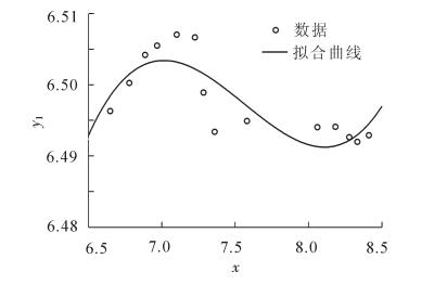
$$ \begin{array}{l} {\rm{ }}{\mathit{y}_{\rm{1}}}{\rm{ = ln}}{\mathit{Y}_{\rm{1}}}{\rm{ = 3}}{\rm{.156 2ln}}\mathit{X}{\rm{-0}}{\rm{.149 6(ln}}\mathit{X}{{\rm{)}}^{\rm{2}}}{\rm{ + 0}}{\rm{.018 5(ln}}\mathit{X}{{\rm{)}}^{\rm{3}}}{\rm{ + 1}}{\rm{.373 4;}}\\ {\mathit{y}_{\rm{2}}}{\rm{ = ln}}{\mathit{Y}_{\rm{2}}}{\rm{ = 29}}{\rm{.513 3ln}}\mathit{X}{\rm{-3}}{\rm{.836 3(ln}}\mathit{X}{{\rm{)}}^{\rm{2}}}{\rm{ + 0}}{\rm{.167 5(ln}}\mathit{X}{{\rm{)}}^{\rm{3}}}{\rm{ + 66}}{\rm{.234}}\;{\rm{7}} \end{array} $$ 从表 8可看出:判定系数R-squared分别为0.714 1和0.988 9, 拟合效果良好, P值在99%的置信水平下显著。从图 1和图 2可看出:数据点均在离拟合曲线上方或下方的不远处, 拟合良好。从残差置信区间(图 3和图 4)可以看出:只有极个别残差的置信区间不含零值, 可剔除。
表 8 回归分析
Table 8. Regression analysis
变量 判定系数 F P y1 0.714 1 9.156 2 0.002 5*** y2 0.988 9 325.388 9 0.000 0*** ***表示在1%的显著性水平通过检验 
图 1 林地面积与林业总产值曲线拟合图
Figure 1. Forest land areaand forestry total production curve fitting

图 2 森林蓄积与林业总产值曲线拟合图
Figure 2. Forest stock and forestry total production curve fitting

图 3 林地面积与林业总产值拟合曲线的残差置信区间图
Figure 3. Residual confidence intervals of forest land areaand forestry total production fitting curve

图 4 森林蓄积与林业总产值拟合曲线的残差置信区间图
Figure 4. Residual confidence intervals of forest stock and forestry total production fitting curve
通过对EKC基本计量模型进行拟合, 拟合曲线良好。从图 1和图 2可看出:林地面积与林业总产值、森林蓄积与林业总产值的曲线均呈“N”型, 趋势上略有不同, 林地面积与林业总产值呈“增—减—增”的发展态势, 林地面积已经过了面积减少的阶段, 即将开始新的上升阶段; 而森林蓄积与林业总产值呈“增—缓—增”的态势, 森林蓄积正处于“N”型曲线的新上升阶段。
通过时间序列对应利用EKC模型拟合的曲线可以看出:“十五”期间(2001-2005年)随着林业经济增长, 林地面积增长, 森林蓄积增长; “十一五”期间(2006-2010年), 随着林业经济增长, 林地面积减少, 森林蓄积增长相对放缓; “十二五”期间(2010-2015年), 随着林业经济增长, 林地面积由减转增, 蓄积增长相对加速。期间森林资源增长放缓与2008年重大雪灾有关, 不得不增加清理灾害林木采伐限额, 减少经济损失。总体来看, 目前森林资源与林业产业基本趋于良性互动, 即将进入“共赢”阶段。
-
从目前来看, 森林资源与林业产业协调向好, 这与当前有效的林业政策和产业调整密不可分。浙江省以“建成森林浙江”为战略目标, 坚持走“绿水青山就是金山银山”的现代林业发展道路, 通过减少林木采伐, 以高效生态复合经营模式提升经营水平, 通过精深加工提高林产品附加值, 加快发展森林休闲养生产业等高效生态富民产业, 推动产业转型升级, 在不破坏森林资源的同时获得经济效益, 提高产值的同时促进了森林资源增长。因此可延续之前的产业政策, 加快一、二、三产业的融合发展, 更好实现林业产业和森林资源的可持续发展。受限于数据资料的相对匮乏, 本研究只考虑了林地面积、森林蓄积2个森林资源指标, 在今后的研究中应加入森林采伐、林产品流通、林产品贸易等其他相关指标, 考虑区域森林资源的流动性, 以及森林资源与林业产业关系可能存在的滞后性。
Dynamic relationship between forest resources and forestry industry: an empirical analysis based on environmental Kuznets curve model
-
摘要: 为更好发展林业产业,同时合理利用森林资源,对森林资源与林业产业的关系进行了研究。基于环境库兹涅茨曲线(environmental Kuznets curve,EKC)模型假设,使用2001-2015年浙江省相关时间序列数据,以林地面积、森林蓄积测度森林资源,林业总产值测度林业产业,在EKC基础计量模型的基础上,对数据进行平稳性检验和协整检验,检验发现变量存在协整关系。在此基础上,分别对林地面积、森林蓄积与林业总产值进行拟合和回归分析,拟合效果良好。结果显示:林地面积与林业总产值、森林蓄积与林业总产值的曲线均呈"N"型,趋势上略有不同,林地面积与林业总产值呈"增-减-增"的发展态势,而森林蓄积与林业总产值呈"增-缓-增"的发展态势。总体上来看,目前森林资源与林业产业趋于良性互动,即将进入"共赢"阶段。Abstract: In order to better develop the forest industry, make rational use of forest resources and provide a reference for forestry development, the research drew on the assumption of environmental Kuznets curve (EKC) model and used the relevant time series data of Zhejiang Province between 2001 and 2015 to build a mathematical model. The forest resources were measured by forest land area, and forest stock; the forestry industry was measured by forestry total production. Based on basic EKC quantitative model, the research conducted stationary test and co-integration test of the data. The research findings indicated that the co-integration relationship existed between forestry total production and forest land area, forest stock relatively. Then on this basis, forest land area and forest stock were respectively compared with forestry total production, and made regression analysis. The analysis found the fitting effect was good. The results showed that the curves of forest land area and forestry total production, forest stock and forestry total production both showed N-shaped, but the trends were slightly different. The trend of forest land area and forestry total production was "increase-decrease-increase", while the forest stock and forestry total production was "increase-gently increase-increase". On the whole, the current forest resources and forestry industry tend to have benign interaction and they are about to enter into the new stage of mutual benefits.
-
Key words:
- forestry economics /
- forest resource /
- forest industry /
- environmental Kuznets curve(EKC)
-
图 1 林地面积与林业总产值曲线拟合图
Figure 1 Forest land areaand forestry total production curve fitting
图 3 林地面积与林业总产值拟合曲线的残差置信区间图
Figure 3 Residual confidence intervals of forest land areaand forestry total production fitting curve
图 4 森林蓄积与林业总产值拟合曲线的残差置信区间图
Figure 4 Residual confidence intervals of forest stock and forestry total production fitting curve
表 1 浙江省林业总产值、林地面积、森林蓄积及对数后的林业产值、林地面积、森林蓄积
Table 1. The data of Zhejiang forestry total production, forest land area, forest stock and the logarithmic data of Zhejiang forestry total production, forest land area, forest stock
年份 总产值X/亿元 林地面积Y1/万hm2 森林蓄积Y2/万m3 x y1 y2 2001 653.72 660.07 13 810.77 6.482 7 6.492 3 9.533 2 2002 769.70 662.71 14 948.22 6.646 0 6.496 3 9.612 3 2003 876.70 665.35 16 085.68 6.776 2 6.500 3 9.685 7 2004 979.27 667.97 17 223.14 6.886 8 6.5042 9.754 0 2005 1 060.74 668.86 18 335.37 6.966 7 6.505 6 9.816 6 2006 1 217.63 669.90 19 381.30 7.1047 6.507 1 9.872 1 2007 1 372.91 669.58 20 235.95 7.224 7 6.506 7 9.915 2 2008 1 457.14 664.46 20 412.06 7.284 2 6.499 0 9.923 9 2009 1 575.89 660.74 21 679.75 7.362 6 6.493 4 9.984 1 2010 1 964.04 661.85 22 763.96 7.582 8 6.4950 10.032 9 2011 3 154.77 661.12 24 091.09 8.056 7 6.493 9 10.089 6 2012 3 576.04 661.27 25 221.55 8.182 0 6.494 2 10.135 5 2013 3 964.72 660.31 26 499.15 8.285 2 6.492 7 10.184 9 2014 4 186.68 659.77 28 114.67 8.339 7 6.491 9 10.244 0 2015 4 522.87 660.49 29 696.98 8.416 9 6.493 0 10.298 8 说明: x=lnX, y1=lnY1, y2=lnY2  下载: 导出CSV
表 2 数据平稳性检验
Table 2. Test series stationarity
变量 ADF检验值 1%临界值 5%临界值 检验结果 y1 -1.833 893 -4.057 910 -3.119 910 未通过检验 y2 -1.687 298 -4.004 425 -3.098 896 未通过检验 x -0.211 113 -4.004 425 -3.098 896 未通过检验
下载: 导出CSV
表 3 变量单位根检验
Table 3. Unit root test
变量 ADF检验值 1%临界值 5%临界值 检验结果 y1 -1.833 893 -4.057 910 -3.119 910 未通过检验 y2 -1.687 298 -4.004 425 -3.098 896 未通过检验 x -0.211 113 -4.004 425 -3.098 896 未通过检验 x2 0.048 931 -4.004 425 -3.098 896 未通过检验 x3 0.274 246 -4.004 425 -3.098 896 未通过检验
下载: 导出CSV
表 4 一阶差分后变量单位根检验
Table 4. Unit root test of first order difference
变量 ADF检验值 1%临界值 5%临界值 检验结果 D(y1) -2.086 624 -4.057 910 -3.119 910 未通过检验 D(y2) -2.736 816 -4.057 910 -3.119 910 未通过检验 D(x) -2.555 699 -4.057 910 -3.119 910 未通过检验 D(x2) -2.534 024 -4.057 910 -3.119 910 未通过检验 D(x3) -2.504 882 -4.057 910 -3.119 910 未通过检验
下载: 导出CSV
表 5 二阶差分后变量单位根检验
Table 5. Unit root test of second order difference
变量 ADF检验值 1%临界值 5%临界值 检验结果 D(y1, 2) -3.438 122 -4.121 990 -3.144 920 通过检验** D(y2, 2) -5.094 094 -4.121 990 -3.144 920 通过检验*** D(x, 2) -3.882 941 -4.121 990 -3.144 920 通过检验** D(x2, 2) -3.929 143 -4.121 990 -3.144 920 通过检验** D(x3, 2) -3.974 993 -4.121 990 -3.144 920 通过检验** 说明:**表示在5%的显著性水平通过检验,***表示在1%的显著性水平通过检验
下载: 导出CSV
表 6 OLS参数估计值
Table 6. OLS estimate of parameter
因变量 变量 系数估计值 t P y1 x 3.156 188 3.144 660 0.009 3*** x2 -0.419 600 -3.091 150 0.010 3** x3 0.018 497 3.033 726 0.011 4** y2 x 29.513 290 3.645 612 0.003 9*** x2 -3.836 292 -3.503 799 0.004 9*** x3 0.167 489 3.405 693 0.005 9*** 说明:**表示在5%的显著性水平通过检验,***表示在1%的显著性水平通过检验
下载: 导出CSV
表 7 残差单位根检验
Table 7. Residual unit root test
残差 ADF检验值 1%临界值 5%临界值 检验结果 r1 -5.016 730 -2.754 993 -1.970 978 通过检验*** r2 -3.434 609 -2.754 993 -1.970 978 通过检验*** 说明:**表示在5%的显著性水平通过检验,***表示在1%的显著性水平通过检验
下载: 导出CSV
表 8 回归分析
Table 8. Regression analysis
变量 判定系数 F P y1 0.714 1 9.156 2 0.002 5*** y2 0.988 9 325.388 9 0.000 0*** ***表示在1%的显著性水平通过检验
下载: 导出CSV
-
[1] 石春娜, 王立群.森林资源消长与经济增长关系计量分析[J].林业经济, 2006(11):46-49. SHI Chunna, WANG Liqun. An econometric analysis on the relations between the growth-declining of forest resources and economic growth[J]. For Econ, 2006(11):46-49. [2] 王馨迪.从我国森林资源现状和林业产值浅论林业经济发展[J].林业科技, 2014, 39(4):57-60. WANG Xindi. Preliminary discuss of the forestry economic development base on the current situation of forest resources and forestry output value in China[J]. For Sci Technol, 2014, 39(4):57-60. [3] 沈月琴, 朱臻, 林建华, 等.浙江省森林资源与林业产业发展的互动关系研究[J].林业资源管理, 2007, 8(4):18-23. SHEN Yueqin, ZHU Zhen, LIN Jianhua, et al. The interaction research on forest resources and forest industry in Zhejiang Province[J]. For Resour Manage, 2007, 8(4):18-23. [4] 李成茂.森林资源培育与林业产业结构及区域布局的关系研究[D].北京: 北京林业大学, 2010. LI Chengmao. The Study on Relationships between Forest Resources Cultivation and Forestry Industrial Structure and Regional Distribution of Forestry Industry[D]. Beijing: Beijing Forestry University, 2010. [5] PANAYOTOU T. Empirical Tests and Policy Analysis of Environmental Degradation at Different Stages of Economic Development[R]. Geneva: International Labour Office, 1993. [6] GROSSMAN G M, KRUEGER A B. Environmental Impact of a North American Free Trade Agreement: Working Paper No.3914[R]. Cambridge: National Bureau of Economic Research, 1991. [7] PANAYOTOU T. Demystifying the environment Kuznets curve:turning a black box into a policy tool[J]. Environ Dev Econ, 1997, 2(4):465-484. [8] CHEN W Y, WANG D T. Economic development and natural amenity:an econometric analysis of urban green spaces in China[J]. Urban For Urban Greening, 2013, 12(4):435-442. [9] AHMED K, SHAHBAZ M, QASIM A, et al. The linkages between deforestation, energy and growth for environmental degradation in Pakistan[J]. Ecol Indic, 2015, 49(2):95-103. [10] MBATU R S. Domestic and international forest regime nexus in Cameroon:An assessment of the effectiveness of REDD + policy design strategy in the context of the climate change regime[J]. For Policy Econ, 2015, 52:46-56. [11] 许姝明.基于环境库兹涅茨曲线假设对中国森林资源变化问题的研究[D].北京: 北京林业大学, 2011. XU Shuming. The Analysis of Forest Resource Change in China based on Environmental Kuznets Curve Assumption[D]. Beijing: Beijing Forestry University, 2011. [12] 李鲁欣.经济增长与林地面积变化的实证分析: 以江西省为例[D].济南: 山东师范大学, 2009. LI Luxin. An Empirical Analysis on the Economic Growth and Change of Woodland Area: Taking Jiangxi Province for an Example[D]. Ji'nan: Shandong Normal University, 2009. [13] 王凯, 陈涛, 罗军伟, 等.基于EKC模型的山东省森林资源变化与人均GDP关系分析[J].林业经济问题, 2016, 36(3):222-226. WANG Kai, CHEN Tao, LUO Junwei, et al. Analysis on the relationship between the change of forest resources and per capita GDP in Shandong Province based EKC model[J]. Issues For Econ, 2016, 36(3):222-226. [14] 史磊, 井晓文.青岛市农业经济增长与面源污染关系研究:基于EKC理论的实证分析[J].山东农业科学, 2016, 48(2):166-169. SHI Lei, JING Xiaowen. Research on dynamic relationship between growth of agricultural output and non-point source pollution in Qingdao:empirical analysis based on environmental Kuznets curve model[J]. Shandong Agric Sci, 2016, 48(2):166-169. [15] 张中华.安徽省农业经济增长与农业面源污染关系的实证研究[J].山西农业大学学报(社会科学版), 2015, 14(4):344-350. ZHANG Zhonghua. An empirical research of the relationship between agricultural economic growth and agricultural non-point source pollution in Anhui Province[J]. J Shanxi Agric Univ Soc Sci Ed, 2015, 14(4):344-350. [16] 付秀梅, 王娜, 项尧尧, 等.海洋经济增长与环境污染水平关系的实证分析[J].中国渔业经济, 2016, 34(5):85-90. FU Xiumei, WANG Na, XIANG Yaoyao, et al. Analysis of relationship between marine economic growth and environmental pollution[J]. Chin Fish Econ, 2016, 34(5):85-90. [17] 赵贺春, 王鹤, 侯思远.我国铝业生产的环境负荷动态分析[J].北方工业大学学报, 2016, 28(4):74-79. ZHAO Hechun, WANG He, HOU Siyuan. A dynamic research on environment load of aluminum production in our country[J]. J North China Univ Technol, 2016, 28(4):74-79. [18] 张锡, 周新苗.浙江省对外贸易发展与环境污染的EKC曲线分析[J].生态经济, 2016, 32(3):80-86. ZHANG Xi, ZHOU Xinmiao. EKC curve analysis of foreign trade development and environmental pollution in Zhejiang Province[J]. Ecol Econ, 2016, 32(3):80-86. [19] 高铁梅, 王金明, 吴桂珍, 等.计量经济分析方法与建模[M].北京:清华大学出版社, 2006:154-157. -

-
链接本文:
https://zlxb.zafu.edu.cn/article/doi/10.11833/j.issn.2095-0756.2018.05.013
 点击查看大图
计量
- 文章访问数: 3762
- HTML全文浏览量: 651
- PDF下载量: 915
- 被引次数: 0
