Volume 41 Issue 4
Jul.  2024
Turn off MathJax
Article Contents

YANG Qiang, LI Xinhao, DU Tao. Comparative study of interpolation methods for missing latent heat flux data[J]. Journal of Zhejiang A&F University, 2024, 41(4): 810-819. doi: 10.11833/j.issn.2095-0756.20230526
Citation: YANG Qiang, LI Xinhao, DU Tao. Comparative study of interpolation methods for missing latent heat flux data[J]. Journal of Zhejiang A&F University, 2024, 41(4): 810-819. doi: 10.11833/j.issn.2095-0756.20230526

Comparative study of interpolation methods for missing latent heat flux data

doi: 10.11833/j.issn.2095-0756.20230526
  • Received Date: 2023-10-24
  • Accepted Date: 2024-04-07
  • Rev Recd Date: 2024-04-04
  • Available Online: 2024-07-12
  • Publish Date: 2024-07-12
  •   Objective  The aim of this study is to analyze and compare the interpolation accuracy of different interpolation methods for missing latent heat flux value (FLE) in ecosystem.   Method  Eddy-covariance (EC) method was used to continuously monitor FLE and environmental factors of a typical natural deciduous broad-leaved forest ecosystem in Songshan National Nature Reserve, Beijing in 2019. Three interpolation methods, namely marginal distribution sampling method (MDS), linear regression method (REG), and artificial neural network method (ANN) were applied to interpolate the missing FLE data (randomly removed from 0.5 h data), and the relationship between measured FLE, interpolated FLE and environmental factors was analyzed.   Result  All the three interpolation results underestimated the measured FLE, among which ANN interpolation value was the closest to the measured one (R2=0.40). The measured FLE showed an exponential relationship with air temperature (Ta) and saturated vapor pressure deficit (DVP). MDS interpolated the relationship between FLE and Ta and DVP, and was the closest to the measured FLE. All the three interpolation methods changed the sensitivity of FLE to Ta and DVP to varying degrees.   Conclusion  The interpolation results of ANN are the closest to the measured values. The relationship between the results of MDS and environmental factors is the closest to the relationship between measured FLE and environmental factors. Therefore, appropriate interpolation methods should be selected in future research based on the research purpose. [Ch, 5 fig. 1 tab. 41 ref.]
  • [1] SONG Sijing, DING Shan, PANG Chunmei, ZHENG Xiao, WANG Tong, YU Shuquan.  Population structure and spatial distribution pattern of Cyclobalanopsis gracilis in the evergreen and deciduous broad-leaved forest in Mount Tianmu . Journal of Zhejiang A&F University, 2023, 40(5): 1073-1081. doi: 10.11833/j.issn.2095-0756.20220784
    [2] ZHENG Xiao, WANG Tong, PANG Chunmei, SONG Sijing, DING Shan, YU Shuquan.  Dynamic study on tree layer of deciduous broad-leaved forest in Mount Tianmu from 1996 to 2017 under climate change . Journal of Zhejiang A&F University, 2023, 40(6): 1250-1260. doi: 10.11833/j.issn.2095-0756.20230185
    [3] GONG Yuan, JI Xiaofang, HUA Yuting, ZHANG Yinlong, LI Nan.  Research progress of CO2 flux in forest ecosystem based on eddy covariance technique: a review . Journal of Zhejiang A&F University, 2020, 37(3): 593-604. doi: 10.11833/j.issn.2095-0756.20190412
    [4] XU Rui, JIANG Chunqian, BAI Yanfeng, LIU Xiuhong, WANG Silong.  Soil greenhouse gas fluxes in pure and mixed stands of Chinese fir . Journal of Zhejiang A&F University, 2019, 36(2): 307-317. doi: 10.11833/j.issn.2095-0756.2019.02.012
    [5] XU Qinghua, YANG Jinliang, HUANG Lianzhong, ZHANG Xingyuan, TAN Xuelian, ZHANG Lu.  Influence of canopy structure on understory vegetation of secondary evergreen broadleaf forest communities . Journal of Zhejiang A&F University, 2019, 36(6): 1151-1157. doi: 10.11833/j.issn.2095-0756.2019.06.012
    [6] LIU Xiaoxiao, DAI Wei, DAI Aona.  Soil enzyme activity and their kinetics in broadleaf forests of Beijing mountainous areas . Journal of Zhejiang A&F University, 2018, 35(5): 794-801. doi: 10.11833/j.issn.2095-0756.2018.05.002
    [7] ZHU Yuyi, XIE Weijia, HUANG Huaguo.  Modeling sensible flux and latent flux in Heihe and boreal forests based on a 3D ENVI-met model . Journal of Zhejiang A&F University, 2018, 35(3): 440-452. doi: 10.11833/j.issn.2095-0756.2018.03.007
    [8] CHEN Liping, LI Pingheng, MO Lufeng, ZHOU Guomo, LI Jinrong.  Carbon flux extraction for a Phyllostachys violascens ecosystem based on the flux footprint analysis . Journal of Zhejiang A&F University, 2016, 33(1): 1-10. doi: 10.11833/j.issn.2095-0756.2016.01.001
    [9] NIU Xiaodong, JIANG Hong, FANG Chengyuan, CHEN Xiaofeng, SUN Heng.  Water vapor flux features of an evergreen and deciduous broadleaf mixed forest in Mount Tianmu area . Journal of Zhejiang A&F University, 2016, 33(2): 216-224. doi: 10.11833/j.issn.2095-0756.2016.02.005
    [10] XU Jian, WEI Xinliang, WANG Jing, WANG Xianting, YU Lipeng.  Intraspecific and interspecific competition of dominant species in a deciduous, broadleaf forest of Longwang Mountain . Journal of Zhejiang A&F University, 2014, 31(6): 868-876. doi: 10.11833/j.issn.2095-0756.2014.06.007
    [11] LIN Enjie, JIANG Hong, CHEN Yunfei.  Water vapor flux variation and net radiation for a Phyllostachys violascens stand in Taihuyuan . Journal of Zhejiang A&F University, 2013, 30(3): 313-318. doi: 10.11833/j.issn.2095-0756.2013.03.001
    [12] DU Hua-qiang, TANG Meng-ping, CUI Rui-rui.  Spatial heterogeneity of soil nutrients in an evergreen broadleaved forest of Mount Tianmu,Zhejiang . Journal of Zhejiang A&F University, 2011, 28(4): 562-568. doi: 10.11833/j.issn.2095-0756.2011.04.007
    [13] YANG Guo-ping, GONG He-de, ZHENG Zheng, ZHANG Yi-ping, LIU Yu-hong, LU Zhi-yun.  Caloric values and ash content of six dominant tree species in an evergreen broadleaf forest of Ailaoshan,Yunnan Province . Journal of Zhejiang A&F University, 2010, 27(2): 251-258. doi: 10.11833/j.issn.2095-0756.2010.02.015
    [14] JIANG Ting, TANG Meng-ping.  Quantitative relationships with competition of dominant tree populations in an evergreen broad-leaved forest on Mount Tianmu . Journal of Zhejiang A&F University, 2008, 25(4): 444-450.
    [15] GONG He-de, ZHANG Yi-ping, LIU Yu-hong, YANG Guo-ping, LU Zhi-yun, LU Hua-zheng.  nterception capability in an evergreen broad-leaved forest of Ailaoshan,Yunnan Province . Journal of Zhejiang A&F University, 2008, 25(4): 469-474.
    [16] FANG Guo-jing, TANG Meng-ping, ZHANG Xue-lian.  The mingling index with evergreen broadleaf forests on Mount Tianmu . Journal of Zhejiang A&F University, 2008, 25(2): 216-220.
    [17] JIN Ze-xin.  Dominant population structure and trend of deciduous broad-leaved forest in the Tiantai Mountains of Zhejiang . Journal of Zhejiang A&F University, 2001, 18(3): 245-251.
    [18] YU Yi-wu, JIANG Zhi-biao, HU Yong-xu.  Stand characteristerics of evergreen broad-leaved forest with Schima superba in Hangzhou . Journal of Zhejiang A&F University, 1999, 16(3): 242-246.
    [19] Lin Kaimin, Lin Guoqing, Zhang Shenlong, Yu Lixuan..  Differences of soil Fertility between Nautral Broadleaved Forest and Replanted Chinese Fir Forest. . Journal of Zhejiang A&F University, 1995, 12(2): 221-225.
    [20] Chen Guorui, Ye Lin, Wang Wei, Yu Yiwu, Li Tianyou..  Regulation Effects of Two Kinds of Forests in Northern Zhejiang on Temperature and Humidity . Journal of Zhejiang A&F University, 1994, 11(2): 143-150.
  • [1]
    FRANK D, REICHSTEIN M, BAHN M, et al. Effects of climate extremes on the terrestrial carbon cycle: concepts, processes and potential future impacts [J]. Global Change Biology, 2015, 21(8): 2861 − 2880.
    [2]
    JIANG Peng, LIU Hongyan, PIAO Shilong, et al. Enhanced growth after extreme wetness compensates for post-drought carbon loss in dry forests [J/OL]. Nature Communications, 2019, 10: 195[2023-09-24]. doi: 10.1038/s41467-018-08229-z.
    [3]
    MATSUMOTO K, OHTA T, NAKAI T, et al. Energy consumption and evapotranspiration at several boreal and temperate forests in the Far East [J]. Agricultural and Forest Meteorology, 2008, 148(12): 1978 − 1989.
    [4]
    MCCAUGHEY J H, PEJAM M R, ARAIN M A, et al. Carbon dioxide and energy fluxes from a boreal mixedwood forest ecosystem in Ontario, Canada [J]. Agricultural and Forest Meteorology, 2006, 140(1/4): 79−96.
    [5]
    KUME T, TANAKA N, KURAJI K, et al. Ten-year evapotranspiration estimates in a Bornean tropical rainforest [J]. Agricultural and Forest Meteorology, 2011, 151(9): 1183 − 1192.
    [6]
    XIE Jing, ZHA Tianshan, ZHOU Caixian, et al. Seasonal variation in ecosystem water use efficiency in an urban-forest reserve affected by periodic drought [J]. Agricultural and Forest Meteorology, 2016, 221: 142 − 151.
    [7]
    WU Jiabing, GUAN Dexin, HAN Shijie, et al. Energy budget above a temperate mixed forest in northeastern China [J]. Hydrological Processes, 2007, 21(18): 2425 − 2434.
    [8]
    WILSON K B, GOLDSTEIN A, FALGE E, et al. Energy balance closure at flux net sites [J]. Agricultural and Forest Meteorology, 2002, 113: 223 − 243.
    [9]
    HUANG Jianping, YU Haipeng, GUAN Xiaodan, et al. Accelerated dryland expansion under climate change [J]. Nature Climate Change, 2016, 6: 166 − 171.
    [10]
    FORNER A, VALLADARES F, BONAL D, et al. Extreme droughts affecting mediterranean tree species’ growth and water-use efficiency: the importance of timing [J]. Tree Physiology, 2018, 38(8): 1127 − 1137.
    [11]
    BALDOCCHI D, FALGE E, GU Lianhong, et al. FLUXNET: a new tool to study the temporal and spatial variability of ecosystem-scale carbon dioxide, water vapor, and energy flux densities [J]. Bulletin of the American Meteorological Society, 2001, 82: 2415 − 2434.
    [12]
    PAPALE D, VALENTINI R. A new assessment of European forests carbon exchanges by eddy fluxes and artificial neural network spatialization [J]. Global Change Biology, 2003, 9(4): 525 − 535.
    [13]
    JIA Xin, ZHA Tianshan, GONG Jinnan, et al. Energy partitioning over a semi-arid shrubland in northern China [J]. Hydrological Process, 2016, 30(6): 972 − 985.
    [14]
    HANSON P J, AMTHOR J S, WULLSCHLEGER S D, et al. Carbon and water cycle simulations for an upland oak forest using 13 stand-level models: intermodel comparisons and evaluations against independent measurements [J]. Ecological Monographs, 2004, 74(3): 443 − 489.
    [15]
    GONG Jinnan, JIA Xin, ZHA Tianshan, et al. Modeling the effects of plant-interspace heterogeneity on water-energy balances in a semiarid ecosystem [J]. Agricultural and Forest Meteorology, 2016, 221: 189 − 206.
    [16]
    GONG Jinnan, WANG Ben, JIA Xin, et al. Modelling the diurnal and seasonal dynamics of soil CO2 exchange in a semiarid ecosystem with high plant-interspace heterogeneity [J]. Biogeosciences, 2018, 15(1): 115 − 136.
    [17]
    WUTZLER T, LUCAS-MOFFAT A, MIGLIAVACCA M, et al. Basic and extensible post-processing of eddy covariance flux data with REddyProc [J]. Biogeosciences, 2018, 15(16): 5015 − 5030.
    [18]
    JIA Xin, MU Yu, ZHA Tianshan, et al. Seasonal and interannual variations in ecosystem respiration in relation to temperature, moisture, and productivity in a temperate semi-arid shrubland [J/OL]. Science of the Total Environment, 2020, 709: 136210[2023-09-24]. doi: 10.1016/j.scitotenv.2019.136210.
    [19]
    FALGE E, TENHUNEN J, BALDOCCHI D, et al. Phase and amplitude of ecosystem carbon release and uptake potentials as derived from FLUXNET measurements [J]. Agricultural and Forest Meteorology, 2002, 113(1/4): 75 − 95.
    [20]
    MA Jingyong, ZHA Tianshan, JIA Xin, et al. Energy and water vapor exchange over a young plantation in northern China [J]. Agricultural and Forest Meteorology, 2019, 263: 334 − 345.
    [21]
    LIU Peng, BLACK T A, JASSAL R S, et al. Divergent long-term trends and interannual variation in ecosystem resource use efficiencies of a southern boreal old black spruce forest 1999−2017 [J]. Global Change Biology, 2019, 25(9): 3056 − 3069.
    [22]
    PASTORELLO G, TROTTA C, CANFORA E, et al. The FLUXNET2015 dataset and the ONEFlux processing pipeline for eddy covariance data [J/OL]. Scientific Data, 72 [2023-09-24]. doi: 10.1038/s41597-021-00851-9.
    [23]
    BARR A G, BLACK T A, HOGG E H, et al. Climatic controls on the carbon and water balances of a boreal aspen forest, 1994−2003 [J]. Global Change Biology, 13(3): 561−576.
    [24]
    BALDOCCHI D, KNOX S, DRONOVA I, et al. The impact of expanding flooded land area on the annual evaporation of rice [J]. Agricultural and Forest Meteorology, 2016, 223: 181 − 193.
    [25]
    TSURUTA K, KOSUGI Y, TAKANASHI S, et al. Inter-annual variations and factors controlling evapotranspiration in a temperate Japanese cypress forest [J]. Hydrological Process, 2016, 30(26): 5012 − 5026.
    [26]
    MIAO Haixia, CHEN Shiping, CHEN Jiquan, et al. Cultivation and grazing altered evapotranspiration and dynamics in Inner Mongolia steppes [J]. Agricultural and Forest Meteorology, 2009, 149(11): 1810 − 1819.
    [27]
    POWELL T L, STARR G, CLARK K L, et al. Ecosystem and understory water and energy exchange for a mature, naturally regenerated pine flatwoods forest in north Florida [J]. Canadian Journal of Forest Research, 2005, 35: 1568 − 1580.
    [28]
    PAPALE D, REICHSTEIN M, AUBINET M, et al. Towards a standardized processing of net ecosystem exchange measured with eddy covariance technique: algorithms and uncertainty estimation [J]. Biogeosciences, 2006, 3(4): 571 − 583.
    [29]
    REICHSTEIN M, FALGE E, BALDOCCHI D, et al. On the separation of net ecosystem exchange into assimilation and ecosystem respiration: review and improved algorithm [J]. Global Change Biology, 2005, 11(9): 1424 − 1439.
    [30]
    AMIRO B D, BARR A G, BLACK T A, et al. Carbon, energy and water fluxes at mature and disturbed forest sites Saskatchewan, Canada [J]. Agricultural and Forest Meteorology, 2006, 136(3/4): 237 − 251.
    [31]
    BURBA G G, MCDERMITT D K, GRELLE A, et al. Addressing the influence of instrument surface heat exchange on the measurements of CO2 flux from open-path gas analyzers [J]. Global Change Biology, 2008, 14(8): 1854 − 1876.
    [32]
    MAUDER M, CUNTZ M, DRÜE C, et al. A strategy for quality and uncertainty assessment of long-term eddy-covariance measurements [J]. Agricultural and Forest Meteorology, 2013, 169: 122 − 135.
    [33]
    WU Xianing, HU Tiesong, WANG Xiugui, et al. Review of estimating and measuring regional evapotranspiration [J]. Transactions of the Chinese Society of Agricultural Engineering, 2006, 22(10): 257 − 262.
    [34]
    WANG Yining, ZHANG Xiaomeng, LU Lu, et al. Estimation of crop coefficient and evapotranspiration of summer maize by path analysis combined with BP neural network [J]. Transactions of the Chinese Society of Agricultural Engineering, 2020, 36(7): 109 − 116.
    [35]
    ZHANG Chuan, YAN Haofang, OUE Hiroki, et al. Parameterization of surface soil available moisture and simulation of soil evaporation beneath canopy [J]. Transactions of the Chinese Society of Agricultural Engineering, 2015, 31(2): 102 − 107.
    [36]
    WU Youjie, DU Taisheng. Estimating and partitioning evapotranspiration of maize farmland based on stable oxygen isotope [J]. Transactions of the Chinese Society of Agricultural Engineering, 2020, 36(4): 127 − 134.
    [37]
    LI Xinhao, YAN Huijuan, WEI Tengzhou, et al. Relative changes of resource use efficiencies and their responses to environmental factors in Artemisia ordosica during growing season [J]. Chinese Journal of Plant Ecology, 2019, 43(10): 889 − 898.
    [38]
    GAO Guanlong, FENG Qi, LIU Xiande, et al. Simulating the leaf stomatal conductance of the desert riparian Tamarix ramosissima Ledeb. based on three empirical models [J]. Acta Ecologica Sinica, 2020, 40(10): 3486 − 3494.
    [39]
    ZHOU Wenjun, ZHA Tianshan, JIA Xin, et al. Dynamics of water use efficiency of Artemisia ordosica leaf in growing season in response to environmental factors in Yanchi, Ningxia of northwestern China [J]. Journal of Beijing Forestry University, 2020, 42(7): 98 − 105.
    [40]
    FENG Xinnyan, JIA Xin, HUANG Jinze, et al. Application of ANN-BiLSTM model to long-term gap-filling of carbon flux data in temperate desert shrub [J]. Journal of Beijing Forestry University, 2023, 45(9): 62 − 72.
    [41]
    LIU Jianzhao, ZUO Yunjiang, WANG Nannan, et al. Comparative analysis of two machine learning algorithms in predicting site-level net ecosystem exchange in major biomes [J/OL]. Remote Sensing, 2021, 13(12): 2242[2023-09-24]. doi: 10.3390/rs13122242.
  • 加载中
通讯作者: 陈斌, bchen63@163.com
  • 1. 

    沈阳化工大学材料科学与工程学院 沈阳 110142

  1. 本站搜索
  2. 百度学术搜索
  3. 万方数据库搜索
  4. CNKI搜索

Figures(5)  / Tables(1)

Article views(52) PDF downloads(4) Cited by()

Related
Proportional views

Comparative study of interpolation methods for missing latent heat flux data

doi: 10.11833/j.issn.2095-0756.20230526

Abstract:   Objective  The aim of this study is to analyze and compare the interpolation accuracy of different interpolation methods for missing latent heat flux value (FLE) in ecosystem.   Method  Eddy-covariance (EC) method was used to continuously monitor FLE and environmental factors of a typical natural deciduous broad-leaved forest ecosystem in Songshan National Nature Reserve, Beijing in 2019. Three interpolation methods, namely marginal distribution sampling method (MDS), linear regression method (REG), and artificial neural network method (ANN) were applied to interpolate the missing FLE data (randomly removed from 0.5 h data), and the relationship between measured FLE, interpolated FLE and environmental factors was analyzed.   Result  All the three interpolation results underestimated the measured FLE, among which ANN interpolation value was the closest to the measured one (R2=0.40). The measured FLE showed an exponential relationship with air temperature (Ta) and saturated vapor pressure deficit (DVP). MDS interpolated the relationship between FLE and Ta and DVP, and was the closest to the measured FLE. All the three interpolation methods changed the sensitivity of FLE to Ta and DVP to varying degrees.   Conclusion  The interpolation results of ANN are the closest to the measured values. The relationship between the results of MDS and environmental factors is the closest to the relationship between measured FLE and environmental factors. Therefore, appropriate interpolation methods should be selected in future research based on the research purpose. [Ch, 5 fig. 1 tab. 41 ref.]

YANG Qiang, LI Xinhao, DU Tao. Comparative study of interpolation methods for missing latent heat flux data[J]. Journal of Zhejiang A&F University, 2024, 41(4): 810-819. doi: 10.11833/j.issn.2095-0756.20230526
Citation: YANG Qiang, LI Xinhao, DU Tao. Comparative study of interpolation methods for missing latent heat flux data[J]. Journal of Zhejiang A&F University, 2024, 41(4): 810-819. doi: 10.11833/j.issn.2095-0756.20230526
  • 气候变化及其对生态系统造成的影响已经成为全球变化研究的重点问题[1]。随着气候变化强度的不断加剧,生态系统的结构和功能必定会受到影响[2]。森林生态系统约占陆地生态系统总面积的30%以上,是陆地生态系统的主体[3],有降低大气二氧化碳(CO2)浓度、涵蓄和调节降水、减少地表侵蚀、调节区域小气候等重要作用[37]。因此,在气候变化背景下,研究森林生态系统过程,如生态系统潜热通量(FLE),对深入理解环境因子对生态系统的调控机制具有重要意义[810]

    涡动相关法已成为从小时到年际时间尺度监测生态系统碳、水和能量通量的主要方法,并成为自下而上估算全球生态系统碳、水平衡过程的支柱[1113]。此外,涡度相关数据也越来越多地被用于生态系统模型的校准和验证[1416]。为了定量估计生态系统过程,准确插补由于不利的气象状况或仪器故障等原因造成的缺失数据是非常重要的[1718]。不同插补方法得到的结果可能有很大差别[1921]。目前,大多数研究只关注插补结果,鲜有研究对插补方法进行比较分析,因此,对现有主要插补方法进行比较分析可以更好地理解生态系统对气候变化的响应。

    如今在世界范围内利用涡动相关系统已经建立了许多通量数据集,尽管各大通量网系统(如FLUXNET、加拿大通量网等)建立数据集的数据收集方法得到了统一,但组织间数据处理方法仍有所不同。例如FLUXNET通量网通常采用边缘分布抽样法对缺失数据进行插补[22],而加拿大通量网通常利用线性与非线性回归法对缺失数据进行插补[23]。这导致相关数据可比性不强[2425]。考虑到气候变化强度不断增强,增强通量数据的可比性是定量预测未来全球生态系统水文循环和改善森林管理决策的关键。

    生态系统蒸散发(ET)作为全球水循环的第二大组成部分,在生态系统内部与外界进行能量和物质交换过程中发挥着重要作用,同时还影响着许多其他重要的生态过程[2627]。本研究于北京松山自然保护区生态环境及生物多样性监测站开展,以天然落叶阔叶林生态系统为研究对象,通过涡度相关法连续监测数据,分析比较落叶阔叶林生态系统FLE缺失值插补的不同方法。本研究假设:插补结果会低估FLE,同时,不同插补方法得到的FLE模拟值有差异。本研究主要解决以下2个问题:①插补FLE与实测FLE是否存在偏差?②插补FLE与环境因子间关系是否和实测FLE与环境因子间关系相同?

    • 松山自然保护区生态环境及生物多样性监测站位于北京市延庆区松山国家级自然保护区内(40°30′48″N,115°47′11″E),离延庆区张山营镇中心约10 km,离北京中心约104 km,北侧与大海坨自然保护区相邻,东南侧为佛峪口水库。

      研究区属于北温带,气候为大陆性季风气候。研究区受所处地形的影响,气温低,湿度高,是典型的山地气候。降水季节分布不均,保证率低,多年平均降水量为450.0 mm,集中在6—9月;多年平均气温为8.9 ℃,极端最高气温为38.1 ℃,极端最低气温为−28.6 ℃,多年平均无霜期为153 d。2018年12月,以通量塔为中心,在冬奥延庆赛区外围松山国家级自然保护区内设立50 m×50 m的样方(40°53′N,116°18′E,海拔为1161 m)。样地内主要乔木树种为胡桃楸Juglans mandshurica,其他乔木树种为大果榆Ulmus macrocarpa、白蜡Fraxinus chinensis等。灌木以绣线菊Spiraea salicifolia、铁线莲Clematis florida为主。经样地调查,胡桃楸平均胸径为10.96 cm,平均树高为4.71 m;大果榆平均胸径为7.20 cm,平均树高为3.88 m;白蜡平均胸径为7.64 cm,平均树高为3.97 m。

    • 通量监测采用开路式涡度相关系统,仪器初始安装高度为20 m。测量系统主要由三维超声分速仪(WindMaster,Campbell Scientific, Inc. Logan)、开路CO2/H2O红外气体分析仪(7500 DS, Campbell Scientific, Inc. Logan)和数据采集器(CR1000,Campbell Scientific, Inc. Logan)构成。同步测量的气象变量包括:净辐射[四分量辐射仪(CNR-4, Campbell Scientific, Inc. Logan)]、空气温度与湿度[空气温湿度传感器(ATMOS14, Campbell Scientific, Inc, Logan, )]、降雨量[雨量桶(ECRN-100, Campbell Scientific, Inc. Logan)],传感器安装高度均为20 m。采用CR1000数据采集器(CR1000, Campbell Scientific, Inc. Logan)采集气象数据,采样频率与涡度相关监测频率同步。

      通量塔5 m半径内随机布设的5套热通量板(HFP01, Campbell Scientific, Inc. Logan)监测土壤热通量,传感器布设深度为10 cm。土壤温度和土壤含水量(CSW)分别由通量塔5 m半径内随机布设的5套土壤温度传感器(5TM, Campbell Scientific, Inc. Logan)和土壤水分传感器(5TM, Campbell Scientific, Inc. Logan)测定,布设深度为10 cm。采用CR1000数据采集器(CR1000, Campbell Scientific, Inc. Logan)采集土壤监测数据。

    • 使用EddyPro软件(version 4, LI-COR, Lincoln)对原始10 Hz数据进行预处理,处理步骤包括峰值去除、倾斜校正(双轴旋转)、传感器滞后校正、光谱校正、去趋势化和0.5 h通量计算[20]。本研究采用PAPALE等[28]的方法剔除0.5 h通量数据异常值,利用数据相对绝对中位偏差(MAD)的偏离程度识别异常数据。具体如下:

      其中:FLEiFLEi−1FLEi+1分别为第i时刻及其前后时刻的FLE数值,diFLEi在数列中的相对位置,di如果满足以下条件则被定义为异常值:

      其中:z为阈值,不同的z可以用来评价该方法对数据的影响,本研究中z取4[28]Md为数列di的中位数。MAD的计算公式如下:

      通过自举法确定摩擦风速阈值[28],夜间摩擦风速低于阈值的湍流均认为交换不均匀,剔除对应FLE值。本研究中摩擦风速阈值为0.204 m·s−1。另外,为了避免由于红外气体分析仪光路受影响导致的测量误差,光路信号值低于70的数据也被剔除。2019年由于仪表故障、系统维护和质量控制等原因剔除掉的FLE占全年数据的37.96%。

    • 边缘分布抽样法(MDS)通过RStudio 1.1.463中的REddyProc程序包完成[29]。该算法主要分为2种不同的情况:①只缺失主要数据,其他气象数据可用;②部分或所有气象数据缺失。在第1种情况下,搜索7 d时间窗口内相似气象条件下是否存在数值,如果有,用满足条件数值的平均值插补缺失值。其中相似气象条件为总辐射(RG, W·m−2)、空气温度(Ta, ℃)和饱和水汽压差(DVP, Pa)相较于缺失值对应的RGTaDVP变化幅度不超过50 W·m−2、2.5 ℃和500 Pa。如果在7 d时间窗口内没有相似气象条件,则将时间窗口增加到14 d。以此类推。

      在第1种情况下,14 d时间窗口内相似条件下存在数值,插补数据质量为高等;21 d时间窗口内相似条件下存在数值,插补数据质量为中等;28 d时间窗口内相似条件下存在数值,插补数据质量为低等。在第2种条件下,FLE缺失数据的时间间隔小于1 h,插补数据质量为高等;FLE缺失数据的时间间隔小于1 d,插补数据质量为中等;FLE缺失数据的时间间隔大于1 d,插补数据质量为低等。

    • 线性回归法主要采用AMIRO等[30]的方法。缺失值的时间间隔小于2 h采用线性内插法插补,其中夜间数据(即RG<20 W·m−2)设为0。缺失值的时间间隔超过2 h分为生长季和非生长季2种情况。生长季(Ta >0 ℃)采用240个连续数据时间窗口内的FLE与净辐射减去土壤热通量(即可利用能量)线性回归插补,时间窗口每次移动48个时间点(1个时间点为0.5 h)。非生长季(Ta<0 ℃)内采用缺失值前5 d至后5 d对应时间的平均值插补。

    • 人工神经网络(ANN)是一种可以映射输入与输出数据间非线性关系的模型。本研究使用BP神经网络,模型为4层结构。输入层包含用于进行模型预测的自变量,输出层包含需要预测的变量,输入层和输出层由2个隐藏层连接。第1个隐藏层的激励函数为tansig函数,第2个隐藏层的激励函数为线性函数,训练方法为Levenberg-Marquardt。1层中的每个神经节点都与相邻层的所有神经节点相连。第1层隐藏层的神经节点数量范围由下式确定:

      其中:m为第1层隐含层神经节点数,nl为输入层和输出层变量个数,α为1~10的正整数。第2层隐藏层神经元个数为1。

      本研究中输入变量为RGTaDVPCSW。为了强调昼夜造成的影响而加入RG,同时将RG<20 W·m−2的值设置为0。白天输入变量为RGTaDVPCSW;夜晚RG=0,输入变量为TaDVPCSW。本研究采用均方误差(ERMSE)来衡量不同m构建的神经网络模型的优劣(表1)。m=9的神经网络模型的ERMSE最低,故本研究中m取9。

      隐藏层神经元个数均方误差平均值
      12345
      30.009 70.010 00.009 90.009 60.010 00.009 8
      40.009 30.009 80.009 60.009 80.010 00.009 7
      50.009 40.009 90.010 30.009 80.009 90.009 9
      60.009 40.009 40.008 80.009 10.009 30.009 2
      70.008 90.009 30.009 90.009 50.009 60.009 5
      80.009 40.009 20.009 30.008 60.008 70.009 0
      90.008 60.008 80.008 50.009 20.009 10.008 8
      100.009 40.009 00.009 50.009 10.009 10.009 2
      110.009 10.009 10.009 10.008 90.009 30.009 1
      120.009 20.010 00.009 30.009 30.009 10.009 4
        说明: 均方误差下的1、2、3、4、5分别指人工神经网络模拟的重复数(即不同的重复)。

      Table 1.  Result of the fitting of the number of different neurons in ANNs

    • 本研究中涡度相关系统采用开路式红外气体分析仪。为了避免出现冬季由于仪器运作散发热量导致的错误通量[31],数据分析时只使用2019年4月11日至10月27日的数据。

      为了评估3种数据插补方法的优良程度,采用随机取点的方法去除30%的FLE有效实测数据(2019年选定日期内数据共11 040个,其中有效实测数据7 576个,即随机去除其中2 272个数据),分别采用上述3种方法插补。插补完成后与实测数据进行比较。

      由于线性回归法将生长季夜晚FLE的缺失值直接填补为0,为了更好地表现线性回归法的结果,本研究将其分为2种情况:第1种为正常线性回归插补(线性回归法Ⅰ),第2种为去除夜晚FLE数据插补(线性回归法Ⅱ)。

      通过分段平均法分析人为去除的有效实测FLE数据及3种数据插补结果与环境因子间的关系,其中线性回归法采用去除夜间FLE插补数据进行分析。Ta按2.5 ℃分段,即每隔2.5 ℃取1次FLE均值; DVP按0.2 kPa分段,分段平均后再拟合。TaFLE使用指数方程y=aexp(bx)进行拟合,其中yFLExTaab为拟合参数;DVPFLE使用指数-二次方程y=exp(a+bx+cx2)进行拟合,其中yFLExDVPabc为拟合参数。

      指数-二次方程可以很好地模拟FLEDVP增大先升高后降低的趋势,可以根据方程计算出最适DVP (DVPopt)为−b/2c

      除MDS方法使用RStudio软件外,其余所有分析均在MATLAB (Version 7.5.0, The MathWorks)中进行。

    • 研究区2019年空气温度(Ta)、10 cm深度土壤温度(Ts)及净辐射(Rn)日均值的变化特征相似,春、冬季较低,夏、秋季较高。研究期内平均Rn为104.85 W·m−2Rn日均值为−13.93~211.82 W·m−2 (图1A)。研究期内平均Ta为13.25 ℃,Ta日均值为−10.63~25.00 ℃。平均Ts为12.08 ℃,Ts的日均值为−0.34~19.28 ℃ (图1B)。平均DVP为0.71 kPa,日均值为0.02~1.98 kPa (图1C)。研究期内降雨总量为503.3 mm,降雨季节分布不均,降雨大多出现在6—9月,占全年降雨总量的78.4%(图1D)。10 cm深度土壤体积含水量(CSW)季节变化范围为0.129 ~ 0.301 m3·m−3。土壤热通量(G)在春冬季为负值,温度上升后开始逐渐增加,在4月7日达到最大值(11.50 W·m−2),研究期内均值为−12.26 W·m−2

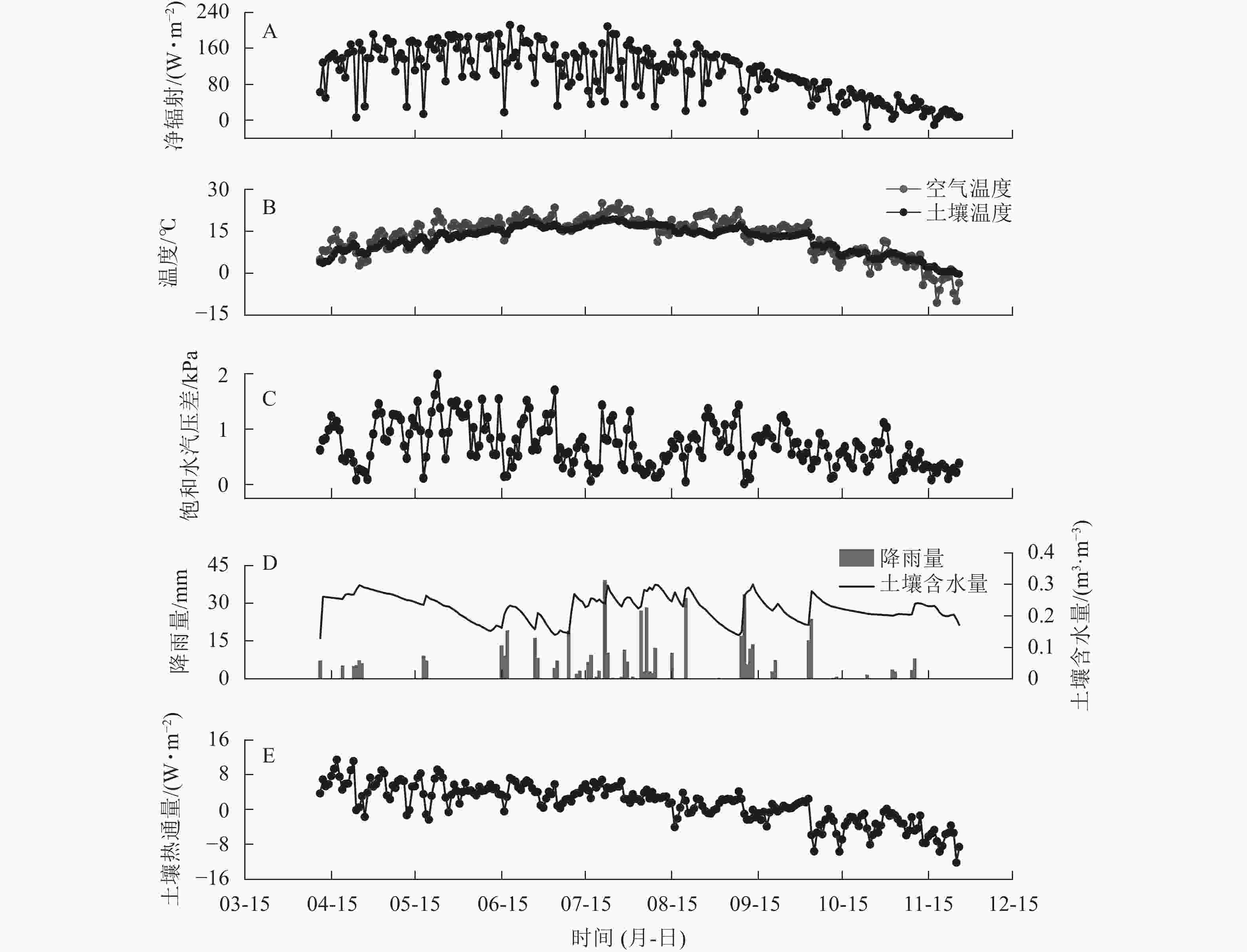
      Figure 1.  Dynamics in daily means of environmental variables in 2019 in the sample plots

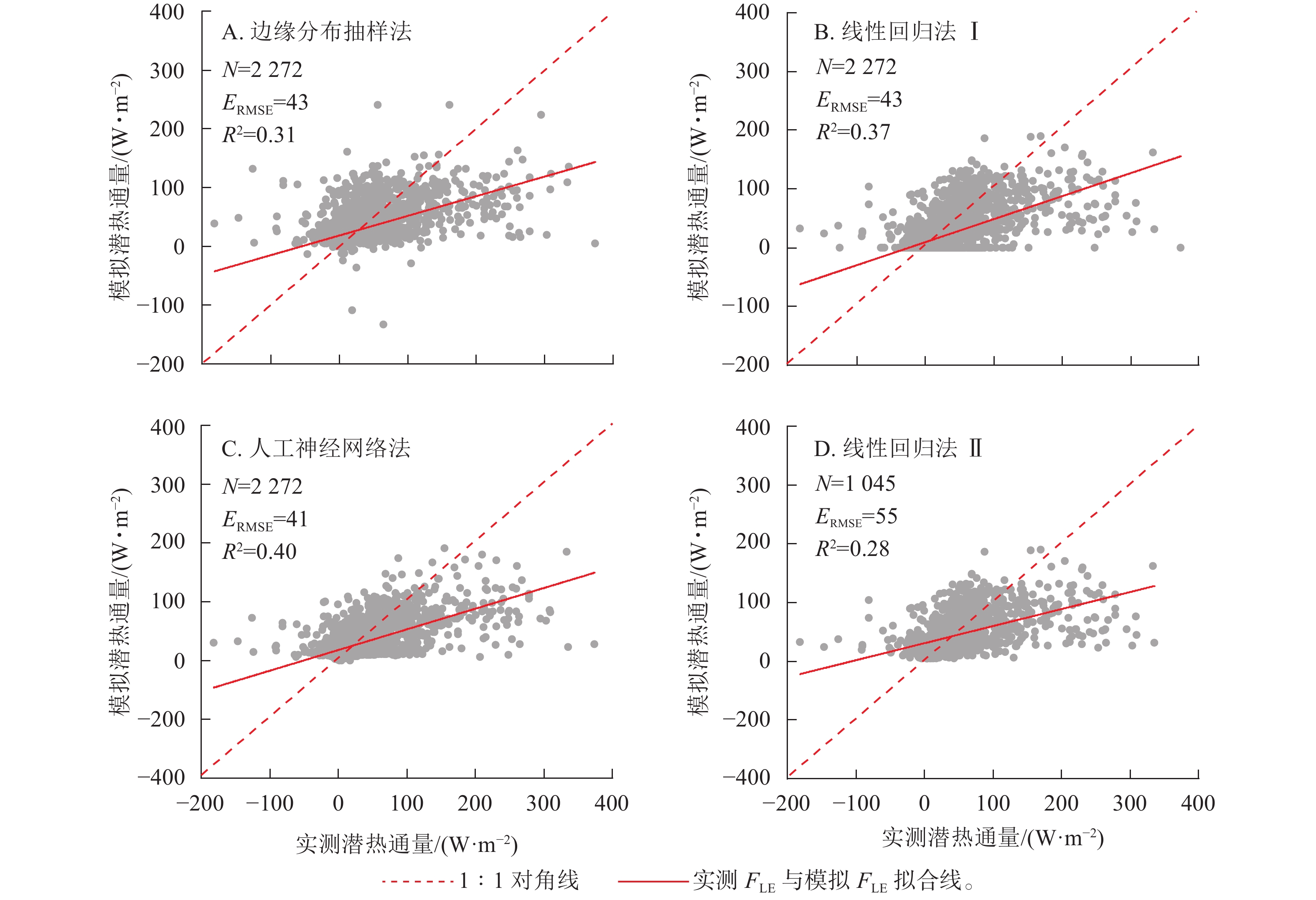
    • 实测FLE与3种插补方法模拟的FLE结果如图2所示,其中插补FLE与实测FLE对比见图3。边缘分布抽样法、线性回归法及人工神经网络法得到的模拟值均低估了FLE,其中决定系数(R2)最高的为人工神经网络法,回归斜率最高的为线性回归法Ⅰ。插补FLE与实测FLE间回归直线截距均在0左右(图3)。

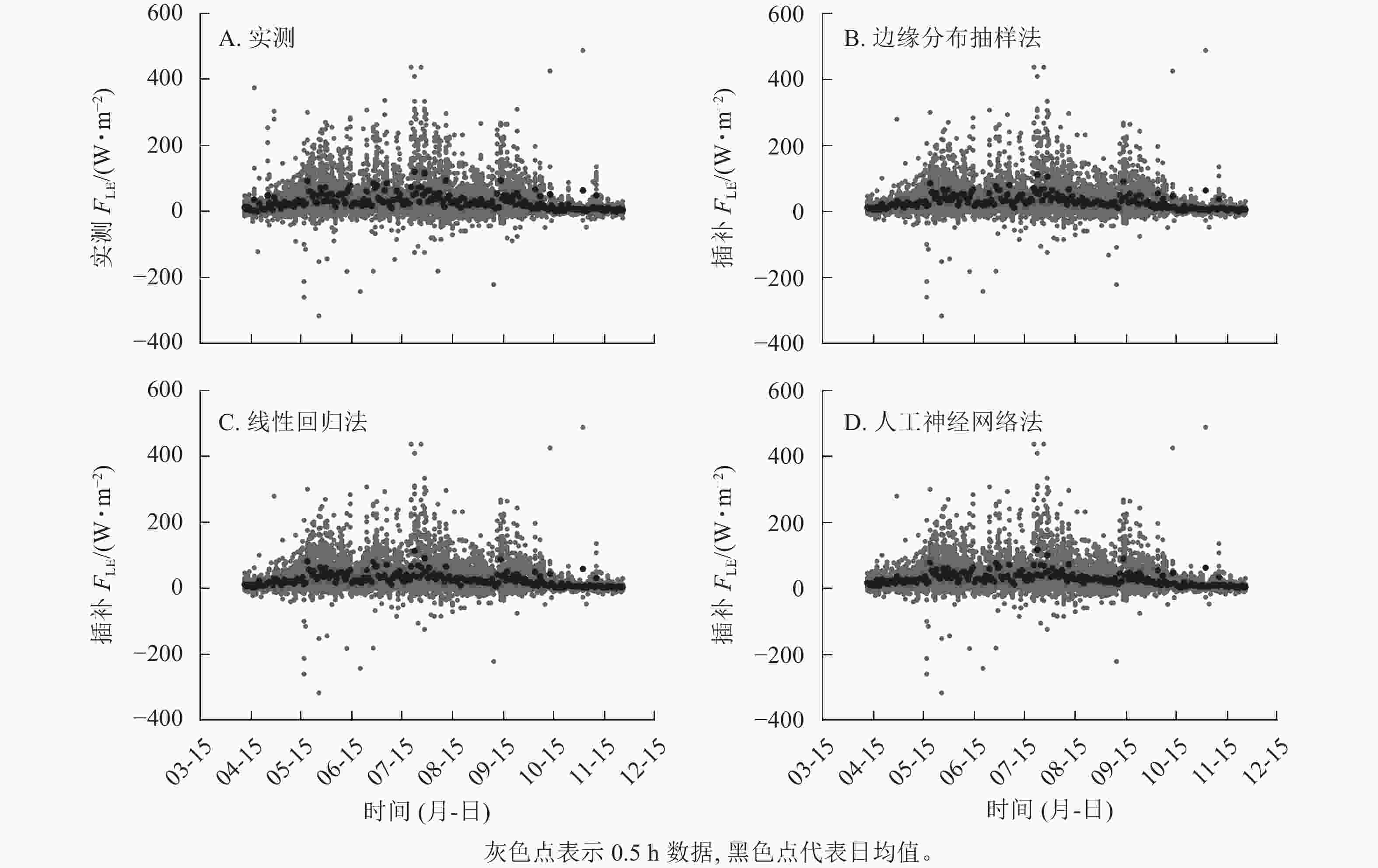
      Figure 2.  Results of measured latent heat flux (FLE) and the modeled FLE with three gap-filling methods in 2019 in the sample plots

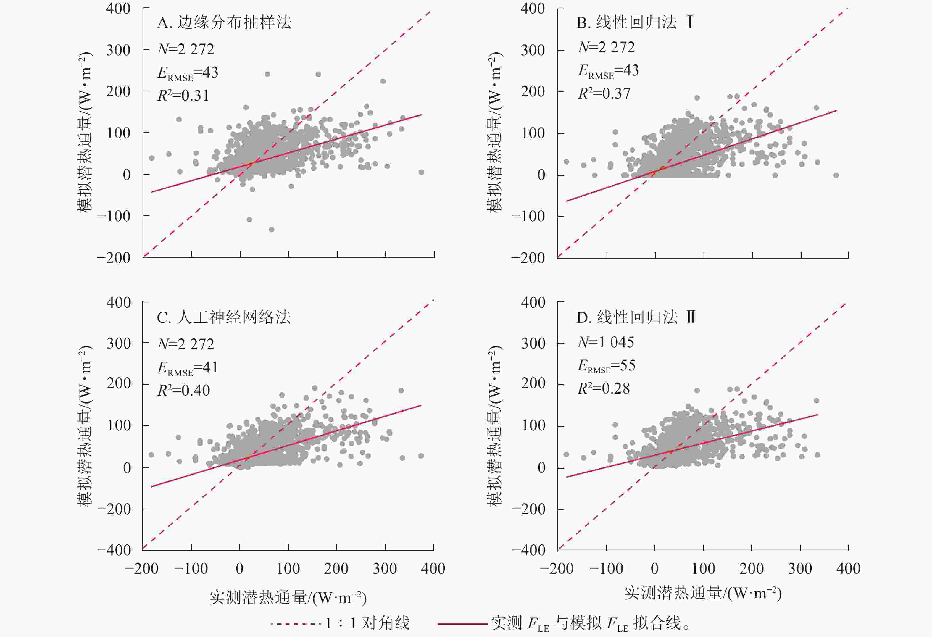
      Figure 3.  Relationship between the measured latent heat flux (FLE) and modeled FLE

      图4所示:3种插补结果中FLETa间拟合参数最接近原始数据的为边缘分布抽样法,拟合效果最好(R2最高)的为边缘分布抽样法。实测FLE及3种插补方法模拟的FLE均随Ta增加而增加,低温时FLETa上升而增加的幅度不大,在15 ℃之后随Ta上升有明显增加。线性回归法插补的FLETa间指数关系不明显。

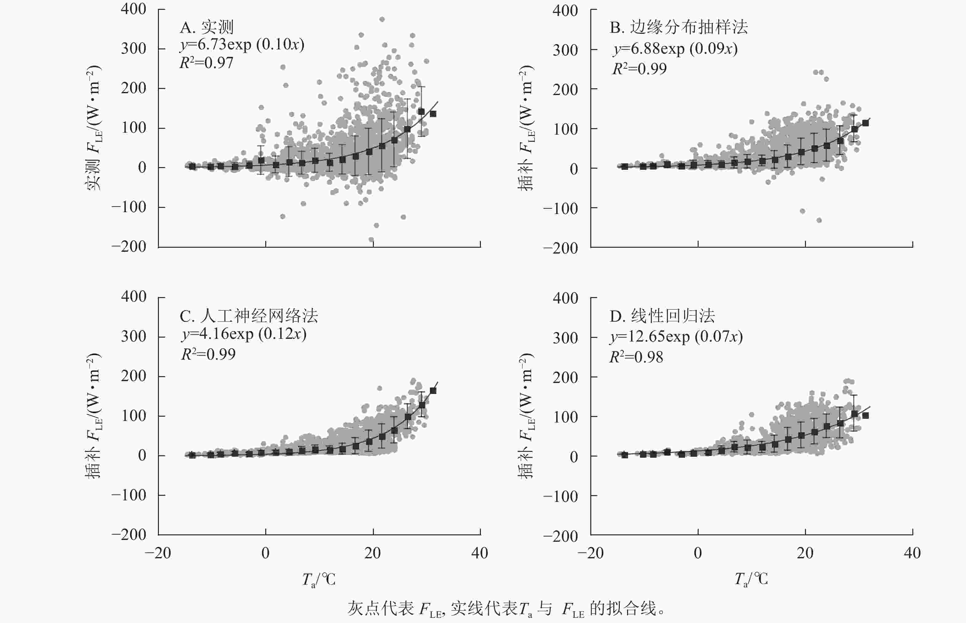
      Figure 4.  Relationship between air temperature (Ta) and measured latent heat flux (FLE) and the three modeled FLE
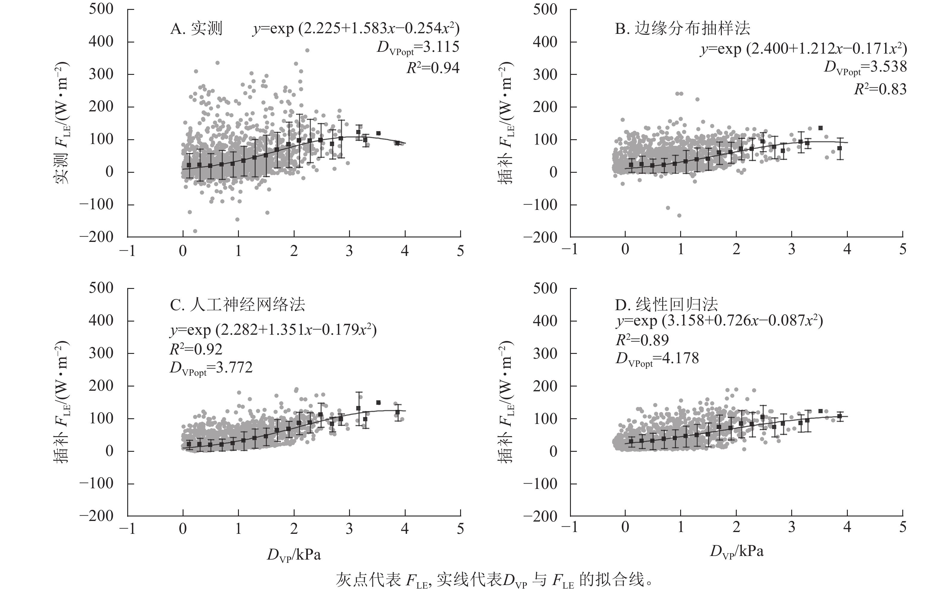
      3种插补结果中,FLEDVP间分段平均后拟合曲线最接近原始数据的为边缘分布抽样法,R2最高的为人工神经网络法(图5)。实测FLE及3种插补FLEDVP间关系均为指数-二次形式,随DVP的增加先增加后减小。实测数据对应的最适DVP(DVPopt)为3.115 kPa,插补结果中DVP最小为边缘分布抽样法,为3.538 kPa,最大DVPopt为线性回归法的4.178 kPa,DVPopt结果与原始数据最接近的为边缘分布抽样法。

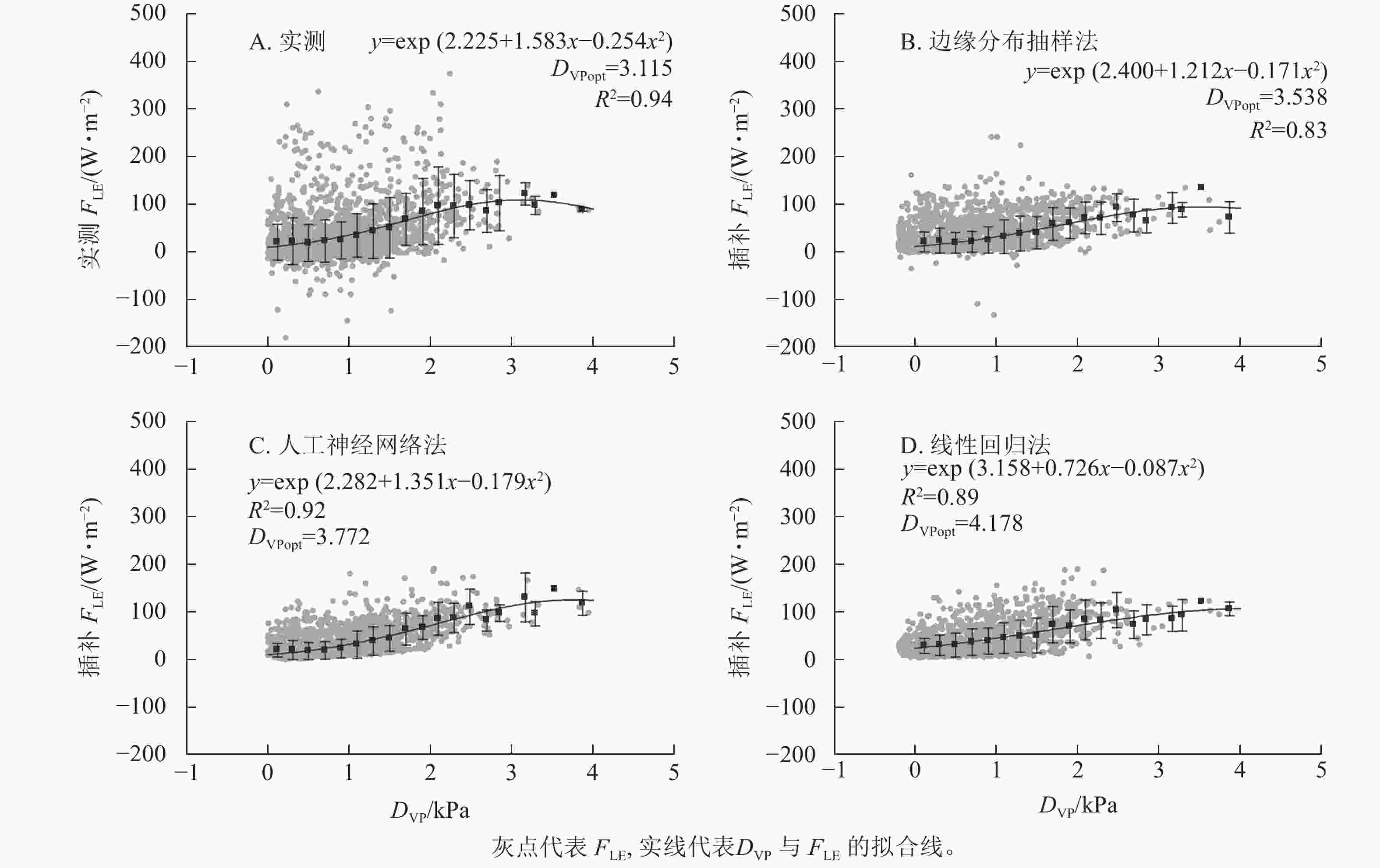
      Figure 5.  Relationship between vapor pressure deficit (DVP) and measured latent heat flux (FLE) and the three modeled FLE

    • 数据插补本质上是在类似气象条件下对有效数据的平均与模拟[8]。本研究中3种插补方法得到的0.5 h数据与实测值间的回归斜率为0.28~0.40,即插补结果与实测FLE相比均有一定程度的低估,其中最接近实测数据的方法为人工神经网络法。涡度相关系统存在随机误差和系统误差(数据采集过程中的错误、仪器自身的偏差及空气的平流运动导致的误差等),监测结果与真实值间会不可避免地出现偏差。该偏差数学分布为标准正态分布,均值为0[32]

      边缘分布抽样法的本质是取类似气象条件下实测有效的平均值进行插补[26],插补值消除了随机偏差,但是这种方法并不能将缓慢变化的生物因素的影响考虑在内(如物候变化)。线性回归法同理。这可能是插补值与实测值间有偏差的原因之一。而人工神经网络法则是利用已有环境数据建模,再根据建立的模型进行反演,建模时已经将原始数据进行了最小二乘回归,即实测值的波动被消除一部分。本研究中插补值与实测值间的比较使用了0.5 h数据,插补值与实测值的日均值间差异可能很小。为了保证插补时有效数据的数量,本研究中无法连续剔除几天数据用于插补,否则会对插补结果造成影响,所以插补结果的日均值是否低估实测值,仍需进一步研究。

    • FLETa呈指数形式。涡度相关中蒸散发由FLE计算得到,蒸散发可以分为土壤蒸发和植物蒸腾2个部分,植物蒸腾主要受水势差控制,而土壤蒸发主要受Ta控制[3334]。本研究中FLETa增加而增加,在气温较低时(<15 ℃) FLETa增加幅度不大,而气温较高时增加幅度变大。这可能是由于气温较低时蒸散发组分增加都不明显,而气温较高时蒸散发开始以土壤蒸发为主,且研究地处于天然森林,土壤中水分充足,所以FLETa增加呈指数形式上升[3536]。3种插补结果中,边缘分布抽样法插补的FLETa间关系与实测值最接近,可能是因为边缘分布抽样法使用了实测数据进行平均插补,可以很好地重现FLETa间的关系。人工神经网络法与线性回归法分段平均后的曲线都与实测数据不符。这可能是因为人工神经网络法是先基于已有数据建模反演,建模时Ta权重较大,所以结果呈明显指数型。线性回归则是利用了RnG间的关系模拟FLE,所以FLETa间关系较差。

      FLEDVP间关系呈指数-二次形式。DVP较低时,FLEDVP增加趋势与Ta类似。DVPTa与相对湿度决定,所以DVP增加会促进生态系统蒸散发上升。随着DVP的不断上升,植被蒸腾失水严重,植物为了保证自身正常生命活动,会主动关闭部分气孔降低自身水分损失,所以随着DVP的不断上升,FLE会先升高后下降[3739]。与Ta相同,边缘分布抽样法与DVP间关系最接近实测值与DVP的关系,人工神经网络法分段平均后FLEDVP整体变化较快,线性回归法没有很好地模拟出FLEDVP先平缓后增加的变化趋势。

    • 3种插补方法各有优缺点,需视具体情况使用。研究表明:人工神经网络通常比其他方法更能准确插补通量缺失数据[4041]。本研究中,将RGTaDVPCSW等影响FLE的主要环境因素作为人工神经网络输入变量,模拟FLE比线性回归与边缘分布抽样法更加贴近实测FLE。人工神经网络法是一种纯经验的“黑箱”模型,其预测能力取决于输入、输出数据集及模型训练过程,输入变量的选择对于其预测能力的影响很大[41]。因此,在预测变量(即气象数据)较全面、监测时序较长的情况下,优先选择人工神经网络对缺失数据进行插补,可以很好地重现FLE动态变化。线性回归法从能量平衡的角度插补数据,这种方法显然没有考虑环境因子对FLE的控制,无法重现与环境因子的关系[29]。边缘分布抽样法将气象条件与FLE的变化同时考虑在内,可以较好地重现与环境因子的关系。因此,尽管线性回归法对FLE动态变化的模拟结果略优于边缘分布抽样法,但是鉴于其对环境因子与FLE关系的重现结果较差,在探究FLE调控机制的研究工作中并不建议使用线性回归法插补FLE缺失数据。当研究中驱动因子有效性不足时,可能需要使用边缘分布抽样法[28];如果插补结果被用于模型验证,为了避免数据与模型间出现虚假或循环关系的现象,可能需要使用线性回归法等[27]

    • ①3种插补方法各有优缺点,得到的插补FLE均对实测FLE有一定低估,人工神经网络法插补结果与实测数据最为接近。②人工神经网络法会过分拟合FLE与环境因子间的关系,线性回归插补结果与环境因子间的关系跟实测数据差别最大,边缘分布抽样法与环境因子间的关系最接近实测FLE

Reference (41)

Catalog

    /

    DownLoad:  Full-Size Img  PowerPoint
    Return
    Return