


-
森林生物量是森林生态系统的核心数据,也是森林碳汇研究的基础[1]。传统生物量获取方法已经不能满足人们对大尺度生物量计算的需求。遥感技术的日益发展,极大提高了森林生物量大尺度估算、及时性掌控和实时性监测的效率。由于Landsat影像不仅能够容易免费获取,而且具有中等的空间分辨率和光谱分辨率以及能够提供较长时间序列的历史数据等优点,被众多学者[2]广泛应用于不同地区不同林分的生物量遥感估测中。基于光学遥感技术估测生物量存在的饱和现象已经受到广泛的关注[3],再加之遥感模型的限制,如线性回归模型普遍存在预估精度不高,模型泛化能力差,估测结果的残差与生物量呈明显的线性关系等问题[2],往往会造成生物量估测的低值高估与高值低估问题,影响了遥感估测生物量精度。虽然一些学者[4-5]通过构建人工神经网络模型和随机森林等非参数机器学习模型提高了线性多变量模型的预估精度,但是由于其“黑箱”操作很难反映生物量与遥感参数之间的机制过程[6],不具有推广性。正是由于混合效应模型包含了固定效应和随机效应2个部分,可以同时分析组水平和个体水平数据,并且在处理不规则及不平衡的分层数据,以及在分析数据的相关性方面具有其他模型无法比拟的优势[7-8]而被广泛使用。曾伟生等[9]利用线性混合效应模型和哑变量模型方法建立了贵州省杉木Cunninghamia lanceolata林和马尾松Pinus massoniana林地上生物量通用性模型。董利虎等[10]为了提高红松Pinus koraiensis人工林枝条生物量模型的精度采用了混合效应模型,并与基础模型的拟合效果进行检验对比。胥喆等[11]采用非线性混合效应模型,选择区域作为随机效应,建立了高山松Pinus densata林生物量估测模型。他们的研究都表明:混合模型各项指标优于一般多变量模型,能有效地提高模型的预估精度。云杉Picea koraiensis和冷杉Abies holophylla均为高海拔地区特有树种,尤其在云南省迪庆藏族自治州广泛分布,占全州森林面积的33.23%[12]。其中云杉为中国西部高山地区特有树种,稍耐阴,耐寒,耐旱,而冷杉常形成纯林,或与性喜冷湿的云杉组成针叶混交林,形成云冷杉林。小班是森林资源清查和经营利用的基本单位,以小班开展研究调查,可以快速、有效、客观地对森林资源变化进行遥感监测,满足时效性与准确性等要求[13]。MOZGERIS[14]和FERNÁNDEZ-MANSO 等[15]的研究均表明:以小班为单位的生物量估算可以提高其精准度。郎晓雪等[16]利用角控样地数据建立云冷杉林蓄积量遥感估测模型的结果值与传统森林资源二类调查数据结果误差仅为1.14%。鉴于此,本研究将基于森林资源二类调查数据结合同时期的Landsat 8 OLI遥感影像,构建不同遥感估测模型,实现对高海拔、大尺度云冷杉林生物量的精确估算,减小生物量遥感估测中低值高估与高值低估的影响,为森林资源二类调查数据广泛利用提供参考和借鉴意义,同时为迪庆区域碳汇效益的准确估算、森林生态保护和科学经营提供规划与指导依据。
-
研究区云南省迪庆藏族自治州,地处26°52′10″~29°15′09″N,98°35′38″~100°18′22″E,属于寒温带气候,平均海拔3 380 m,年平均气温为4.7~16.5 ℃。全州林业用地173.96 万hm2,森林覆盖率高达73.9%,境内主要树种有云杉、冷杉、云南松Pinus yunnanensis、高山松等,是云南省重点林区,森林资源极为丰富,其中云冷杉林面积57.82 万hm2[12]。
-
地面数据。地面数据为云南省迪庆藏族自治州2016年完成的森林资源二类调查数据,包括小班空间位置、面积、起源、优势树种、蓄积量、龄组等基本小班调查因子。
遥感影像数据。由于该地二类调查数据调查时间大多在冬春季,本研究选取与地面数据同时期的空间分辨率为30 m的Landsat 8 OLI遥感影像。数据(表1)来源于中国科学院计算机网络信息中心地理空间数据云平台(http://www.gscloud.cn)。
表 1 研究区Landsat 8 OLI影像基本信息
Table 1. Basic information of Landsat 8 OLI images in study area
影像ID 获取时间 条带号 太阳方位角/(°) 太阳高度角/(°) 平均云量/% LC81310412016341LGN00 2016-12-06 131/041 156.524 36.313 1.04 LC81320402016348LGN00 2016-12-13 132/040 156.677 34.220 0.73 LC81320412016348LGN00 2016-12-13 132/041 156.001 35.443 0.76 数字高程 (DEM)数据与辅助数据。迪庆藏族自治州DEM数据分辨率为30 m。本研究采用的辅助数据为迪庆藏族自治州行政区划矢量图,用来裁剪最终影像。
-
地面生物量数据通过生物量—蓄积量转换来计算。参考胥辉等[12]的云南省迪庆地区云冷杉乔木层生物量—蓄积量转换因子(表2)。
表 2 云冷杉蓄积量—生物量转换因子信息指数
Table 2. Spruce and fir storage—biomass conversion factor information index
树种 模型公式 FBE DSV 幼龄林 中龄林 近熟林 成熟林 过熟林 乔木层 云杉 MA=VFBEDSV 2.326 5 1.516 4 1.473 0 1.427 4 1.264 2 0.342 冷杉 1.327 9 1.339 3 1.333 6 1.309 7 1.285 9 0.366 说明:MA为单位面积生物量;V为单位面积蓄积量;FBE为蓄积生物量转换系数;DSV为木材基本密度 -
首先,从二类调查数据里提取优势树种为云冷杉的小班班块,删除蓄积量为0的异常小班数据,再利用ARCGIS 10.5软件的“采样—创建随机点”工具,设置约束范围1.5 km[17],结果为1 233块。最后进行目视检查,确保云冷杉小班不含其他非植被像元。最终留得1 228块小班样本数据,其中983块小班(80%)用于建模(训练),245块小班(20%)用于独立性检验(表3)。
表 3 建模及检验数据基本情况
Table 3. Modeling and testing data
统计量 建模/训练数据(n=983) 检验数据(n=245) 单位面积蓄
积量/(m3∙hm−2)单位面积生
物量/(t∙hm−2)单位面积蓄
积量/(m3∙hm−2)单位面积生
物量/(t∙hm−2)最小值 8.33 5.74 28.57 14.37 最大值 651.82 314.83 598.92 287.88 平均值 294.73 141.66 298.78 143.57 标准差 137.54 65.43 122.51 58.65 -
本研究采用的遥感数据为Landsat 8 OLI Leve1级别。数据已进行几何粗校正,精度满足研究需求,并对遥感数据进行辐射定标、FLAASH大气校正,消除传感器本身、大气、太阳高度角等带来的干扰,得到真实反射率数据。然后为消除地表阴影对遥感特征值的影响,本研究采用1∶50 000地形图生成的30 m空间分辨率数字高程图进行地形校正,其具体流程方法参照董宇[18]的研究。同时,根据现有迪庆藏族自治州云冷杉林小班矢量边界对遥感影像进行棋盘分割与融合,从而保证2种数据在空间尺度的匹配,最后对影像进行镶嵌和裁剪处理。
遥感因子的提取大致分为4类,包括原始单波段因子、植被指数[19]、归一化植被指数[20]、信息增强因子[19-20](表4)。
表 4 建模变量因子
Table 4. Modeling variable factors
以云冷杉各个小班面状数据为单位,利用ARCGIS 10.5软件的“分区统计”功能,统计每个小班样地内各个遥感因子反射率的最小值(以下称MIN)、最大值(MAX)和平均值(MEAN)。然后进行因子优选,选取与生物量相关性极显著且因子之间相关性小的因子参与到模型的构建中。本研究采用的是皮尔逊相关性检验,采用方差膨胀因子(VIF大于10)解决因子之间的多重共线性问题。
-
本研究通过构建生物量与波段反射率间的散点图,用曲线拟合两者之间的函数关系,计算函数所对应的极值即为生物量遥感估测的数据饱和值。
-
①逐步线性回归模型的构建。利用SPSS 23软件进行线性逐步回归模型的拟合,分别构建生物量与各个遥感因子反射率最小值、最大值和平均值的逐步回归模型,通过偏F统计检验,将自变量一个个引入到模型中;同时,每引进一个新变量,将对已纳入的变量再次进行检验,确保模型中只包含对因变量影响最显著的自变量的最优模型[21]。其基本表达式为:
$$ y={b}_{0}+{b}_{1}{x}_{1}+{b}_{2}{x}_{2}+\cdots +{b}_{n}{x}_{n}+\varepsilon \text{。} $$ (1) 式(1)中:y为生物量因变量;b0为常数项;b1,b2,
$\cdots $ ,bn为拟合参数;x1,x2,$\cdots $ ,xn为自变量;n为自变量个数;ε为随机残差。②BP神经网络模型的构建。本研究在Matlab软件中采用3层BP神经网络,完成模型构建、模型估测及预测值的计算。输入层的神经元个数为回归模型最终优选的自变量,输出层神经元个数为1,隐含层神经元个数参考经验公式(2)选取。网络训练函数采用trainlm,网络最大训练次数为1 000,学习速率为0.01,目标误差选取0.001、0.005、0.010与隐含层神经元个数进行组合训练网络。$$ m=\sqrt{n+l}+a\text{。} $$ (2) 式中(2):m为隐含层神经元个数;n为输入层神经元个数;l为输出层神经元个数;a为1~10的整数。③混合效应模型的构建。利用R语言的nlme模块实现混合效应模型的构建。研究发现:迪庆藏族自治州垂直气候特点显著,在不同区域内森林生物量生长存在随机差异。按迪庆藏族自治州行政区划的各个县(市),分为不同区域,设为第1水平随机效应因子;在不同区域内又嵌套着不同龄组的云冷杉林,设为第2水平随机效应因子,故本研究基于回归模型为基础模型,考虑单水平(区域、龄组)和嵌套两水平(区域+龄组)分别构建云冷杉林生物量线性混合效应模型。其基本形式如下:
$$ \left\{\begin{aligned} & {y}_{ij}={X}_{ij}\beta +{Z}_{i,j}{b}_{i}+{Z}_{ij}{b}_{ij}+{e}_{ij};\;i=1,\cdots ,m;\;j=1,\cdots ,{m}_{i}\\ & {b}_{i} \sim N\left(0,{D}_{1}\right),\;{b}_{ij} \sim N\left(0,{D}_{2}\right)\\ & {e}_{ij} \sim N\left(0,{\sigma }^{2}{R}_{i}\right)\end{aligned}\right.\text{。} $$ (3) 式(3)中:yij为第i个1水平中的第j个2水平内的观察值;m为第1水平的分组数;mi为对应于第1水平的第2水平的分组数;Xij为已知设计矩阵。在本研究中即为最优逐步回归模型;β为固定参数向量;Zi,j和Zij分别为1水平和2水平的随机效应设计矩阵;bi和bij分别为1水平和2水平的随机参数向量;D1和D2分别为1水平和2水平的组间方差-协方差矩阵;σ2为方差;Ri为模型的组内方差-协方差结构;eij为模型的误差项。
根据众多学者的研究[8,10,22-23],完成混合效应模型的构建还需要以下内容。①确定参数效应:本研究将不同随机参数组合的混合模型进行拟合,通过评价模型拟合指标,即比较Akaike信息指数(AIC)、贝叶斯信息指数(BIC)和对数似然值(logLik)参数指标,其中AIC、BIC越小越好,logLik越大越好。②确定组间方差-协方差结构(D矩阵):当随机效应参数的个数大于1时应考虑组间方差-协方差结构。本研究将比较广义正定矩阵(UN)、复合对称结构(CS)和对角矩阵结构(UN1)3种结构对模型的影响。具体形式(以2个随机效应参数为例)如下:
$$ {{{U}}_{\rm{N}}} = \left[ {\begin{array}{*{20}{c}} {{\sigma _1}^2}&{{\sigma _{12}}}\\ {{\sigma _{21}}}&{{\sigma _2}^2} \end{array}} \right]\text{;} $$ (4) $$ {{{C}}_{\rm{S}}} = \left[ {\begin{array}{*{20}{c}} {{\sigma ^2} + {\sigma _1}}&{{\sigma _1}}\\ {{\sigma _1}}&{{\sigma ^2} + {\sigma _1}} \end{array}} \right]\text{;} $$ (5) $$ {{{U}}_{{\rm{N}}1}} = \left[ {\begin{array}{*{20}{c}} {{\sigma _1}^2}&0\\ 0&{{\sigma _2}^2} \end{array}} \right]\text{。} $$ (6) ③确定组内方差-协方差结构(R矩阵):首先要考虑组内误差的异方差性和自相关性问题。为了解决这2个方面问题从而确定组内方差-协方差结构,林业上主要采用式(7)进行描述:
$$ {R}_{i}={\sigma }_{i}^{2}{{\varPsi }}_{i}^{0.5}\times \varGamma _{i}\left(\theta \right)\times {{\varPsi }}_{i}^{0.5}\text{。} $$ (7) 式(7)中:Ri为组内方差-协方差矩阵;σi2为混合模型的误差方差值;Ψi0.5为描述方差异质性的对角矩阵;Γi (θ)为组内误差自相关结构矩阵。
本研究将通过残差分布图来判断误差的异质性。由于本研究所使用的数据不涉及时间序列相关性,故主要测试指数函数(exponential)、高斯函数(Gaussian)和球面函数(spherical)3种空间自相关函数对模型的影响。具体结构形式见文献[24]。④混合效应模型参数估计:在应用混合效应模型时,需要估计随机参数。在本研究中,随机效应参数值可通过建模及检验小班样本数据已知信息,参考VONESH等[25]研究,利用最好线性无偏估计以及限制性极大似然法预测。具体形式如下:
$$ {\hat b}_{i}={{{\hat{D}}}{{{\hat{Z}}}}_{i}^{T}({{{\hat{R}}}}_{i}+{{{\hat{Z}}}}_{i}{{\hat{D}}}{{{\hat{Z}}}}_{i}^{T})}^{-1}{\hat{e}}_{i}\text{。} $$ (8) 式(8)中:
${\hat{b}}_{i}$ 为预估的随机参数值;${{\hat{D} }}$ 为n×n维组间方差-协方差矩阵(n为随机参数个数);${{{\hat{R}}}}_{i}$ 为q×q维组内方差-协方差矩阵;${\hat{e}}_{i}$ 为q×1维误差向量;${{{\hat{Z}}}}_{i}$ 为随机效应设计矩阵。 -
本研究采用调整决定系数(
$ R_{\rm{a}}^2 $ )作为基础模型评价指标,混合效应模型选取logLik值、AIC和BIC作为评价指标。选取总相对误差(RS)和平均相对误差(EE)2个指标对模型进行独立性检验,其具体结构公式见文献[7-8, 19]。采用刀切法分组,依据生物量饱和值将生物量分段处理,选取平均残差(RM)对模型在不同生物量段下的预估能力进行评价分析。$$ {R}_{{\rm{M}}}=\frac{\displaystyle\sum\limits _{i=1}^{n}({y}_{i}-{\bar y}_{i})}{n}\text{。} $$ (9) 式(9)中:
$ {y}_{i} $ 为观测值;$ {\bar y}_{i} $ 为预测值;$ n $ 为样本容量。 -
利用本研究选取的41个遥感因子与样本云冷杉林地上生物量进行Pearson’s相关性分析,结果(表5)可以看出:相较于最大值和最小值反射率平均值与生物量之间相关性更强,其中B6波段的反射率平均值与生物量有最强的相关性,因此,基于B6波段分析和确定云冷杉林的生物量饱和值。
表 5 生物量与遥感因子各统计值相关性
Table 5. Significant Pearson correlation coefficients between remote sensing factors and AGB
遥感因子 MEAN MAX MIN 遥感因子 MEAN MAX MIN ALBEDO −0.555** −0.065* −0.449** ND67 0.439** 0.160** 0.317** ARVI 0.469** 0.251** 0.193** NDVI 0.329** 0.216** 0.069* B −0.540** −0.055 −0.430** NLI 0.165** 0.207** 0.091** B1 −0.168** 0.010 −0.092** PC1-A −0.682** −0.154** 0.323** B2 −0.187** 0.008 −0.097** PC1-B −0.711** −0.165** 0.337** B3 −0.238** 0.001 −0.095** PC1-P 0.616** 0.383** −0.180** B4 −0.334** −0.018 −0.096** PC2-A 0.440** 0.172** −0.110** B5 −0.296** 0.003 −0.100** PC2-B 0.099** 0.040 −0.097** B6 −0.762** −0.333** −0.101** PC2-P 0.670** 0.349** 0.085** B7 −0.705** −0.345** −0.219** PC3-A −0.094** 0.016 −0.004 DVI −0.050 0.036 −0.220** PC3-B −0.039 0.049 −0.470** G 0.057 0.051 −0.203** PC3-P −0.197** 0.006 −0.531** KT1 −0.555** −0.060* −0.203** PVI −0.237** 0.004 0.163** KT2 0.070* 0.053 −0.521** RVI 0.102** −0.002 0.325** KT3 0.534** 0.126** −0.523** SARV −0.036 −0.041 0.176** MSAVI 0.326** 0.215** −0.430** SAV12 0.326** 0.215** 0.361** MSR 0.269** 0.009 −0.430** SAVI 0.329** 0.216** 0.043 MVI5 0.626** 0.436** −0.057* SR 0.102** −0.002 −0.016 MVI7 0.619** 0.363** −0.018 TVI 0.329** 0.217** −0.052 ND43 −0.490** −0.251** −0.441** W 0.497** 0.114** −0.174** ND563 −0.075* 0.010 −0.015 说明:**表示极显著相关(P<0.01);*表示显著相关(P<0.05) -
基于B6波段遥感因子,选取常用含极值函数与生物量进行曲线拟合求解云冷杉林地上生物量饱和值。由表6可知:幂函数拟合时有最高的决定系数R2(0.590),故以其所对应的幂函数极值(图1)作为该波段的云冷杉林生物量饱和值,其值为233 t·hm−2。
表 6 基于不同曲线拟合饱和值结果
Table 6. Results of fitting saturation values based on different curves
函数 R2 P 对数函数 0.555 0.000 二次项函数 0.583 0.000 三次项函数 0.584 0.000 幂函数 0.590 0.000 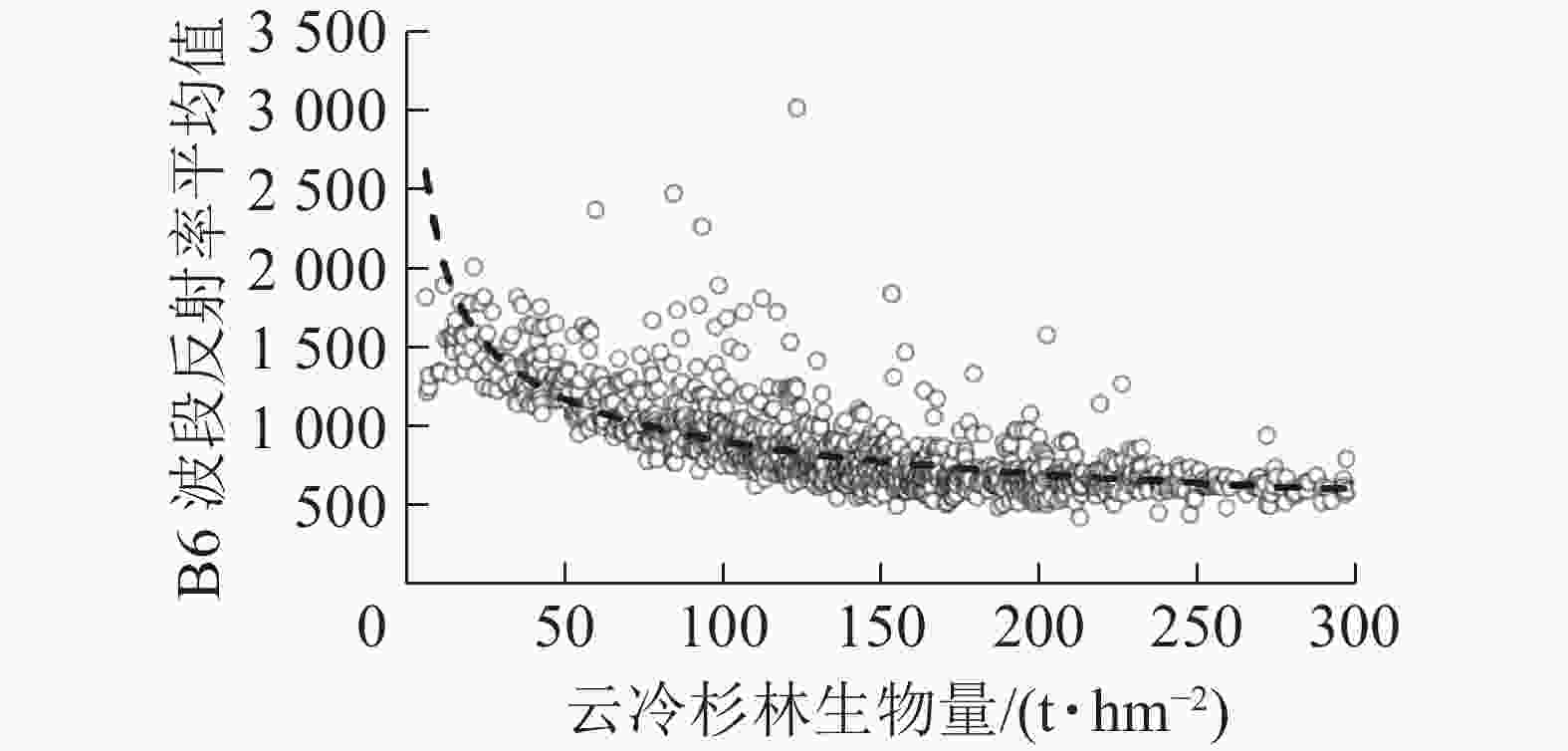
图 1 幂函数拟合云冷杉林生物量饱和曲线
Figure 1. Power function fitting curve of spruce-fir forest biomass saturation
-
通过生物量与各个遥感因子反射率统计值构建的逐步回归模型结果可知,反射率平均值与生物量的回归模型相较于采用最小值和最大值所构建模型的Ra2最高,总相对误差(13.715)和平均相对误差(1.931)也均最优。因此,采用反射率平均值与生物量所构建的逐步回归模型[式(10)]作为BP神经网络输入层神经元个数的纳入依据以及混合效应模型构建的基础模型。
$$ Y=295.75-0.253A+0.182B+120.979C\text{。} $$ (10) 式(10)中:
$ Y $ 为因变量;A为B6波段值;B为B7波段值;C为归一化植被指数(NDVI)。 -
经上节回归模型筛选出的自变量为3个,则经计算隐含层神经元个数的取值范围为[3, 12]的整数。通过对隐含层神经元个数及目标误差的每个不同组合进行10次训练,取平均值。最终隐含层神经元个数与目标误差组合为(6, 0.01)时,Ra2最优(0.542),总相对误差最小(12.190)。
-
确定参数效应和组间方差-协方差结构需要同时进行。首先将组间方差-协方差结构设为默认广义正定结构,拟合结果见表7。基于区域效应水平,共有7种拟合模型,其中有6种模型收敛,混合效应模型相较于基础模型其AIC和BIC值均较小,logLik值均较大,表现出混合效应模型比基本模型有更好的拟合精度,其中模型1有最小的AIC、BIC值和最大的logLik值,即把a1考虑为随机参数的混合模型作为基于区域效应水平的最优模型。基于龄组效应水平,共有7种拟合模型,均收敛,结果见表7。混合模型同样相较于基础模型有着较优的拟合指标,其中模型1有最小的AIC、BIC值和最大的logLik值,即将a1考虑为随机参数的混合模型作为基于龄组效应水平的最优模型。
表 7 基于单水平混合参数选择拟合结果
Table 7. Selection of fitting results based on single-level mixing parameters
模型 混合参数 区域效应 龄组效应 AIC BIC logLik AIC BIC logLik 基础模型 无 10 129.57 10 154.04 −5 059.787 10 129.57 10 154.04 −5 059.787 模型1 a1 10 093.99 10 133.10 −5 038.993 10 011.61 10 050.73 −4 997.806 模型2 a2 10 102.12 10 141.24 −5 043.062 10 016.07 10 055.18 −5 000.034 模型3 a3 不收敛 10 023.89 10 063.00 −5 003.943 模型4 a1, a2 10 099.99 10 153.78 −5 038.996 10 017.62 10 071.41 −4 997.812 模型5 a1, a3 10 100.01 10 153.80 −5 039.007 10 017.66 10 071.44 −4 997.829 模型6 a2, a3 10 108.13 10 161.92 −5 043.066 10 022.21 10 075.99 −5 000.105 模型7 a1, a2, a3 10 108.00 10 181.34 −5 038.998 10 023.67 10 053.00 −5 005.834 -
两水平混合效应模型将同时考虑区域效应和龄组效应。当模型有2个随机参数时,得到9种拟合模型,其中有7种模型收敛;当模型有3个随机参数时,共有18种拟合模型,其中有14种模型收敛;当模型有4个随机参数时,共有15种拟合模型,其中有9种模型收敛;当模型有5个随机参数时,共有6种拟合模型,其中有3种模型收敛;当模型有6个随机参数时,只有1种拟合模型且收敛。由于拟合模型众多,本研究只列出相同随机参数下的最优混合模型,结果见表8。综合分析模型的3个拟合指标,将模型1,即把区域效应含有随机参数a1和龄组效应含有随机参数a1的混合模型作为两水平效应上的最优模型。然后又将林业上使用较为广泛的2种组间方差-协方差结构纳入模型,结果见表9。通过对AIC、BIC、logLik值和似然比检验结果可见,广义正定结构表现较优,因此将两水平混合效应模型的组间方差-协方差结构设为广义正定结构。
表 8 基于两水平混合参数选择拟合结果
Table 8. Selection of fitting results based on two levels of mixing parameters
模型 区域效应 龄组效应 AIC BIC logLik a1 a2 a3 a1 a2 a3 模型1 √ √ 9 956.50 10 010.29 −4 967.250 模型2 √ √ √ 9 958.93 10 012.71 −4 968.464 模型3 √ √ √ √ 9 957.83 10 045.84 −4 960.915 模型4 √ √ √ √ √ 9 963.75 10 066.43 −4 960.872 模型5 √ √ √ √ √ √ 9 971.72 10 093.96 −4 960.862 说明:带√的变量表示模型包含这个随机参数 表 9 基于随机参数不同组间方差-协方差结构混合模型拟合结果
Table 9. Mixed model fitting results of variance-covariance structure between groups based on random parameters
方差-协方差结构 自由度 AIC BIC logLik 似然比检验(LRT) P 广义正定矩阵(UN) 11 9 956.50 10 010.29 −4 967.250 复合对称(CS) 10 9 958.34 10 012.24 −4 969.170 18.396 56 <0.000 1 对角矩阵(UN1) 9 9 965.69 10 009.70 −4 973.846 13.190 81 0.001 4 -
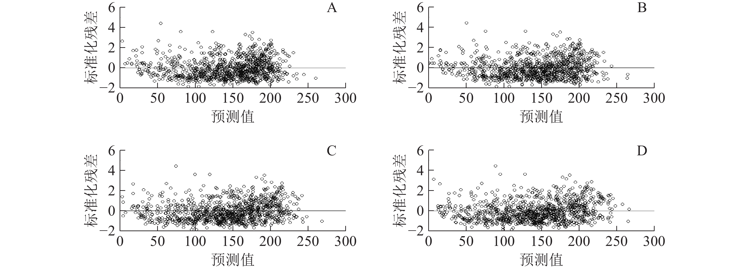
确定组内方差-协方差结构。首先,要确定误差的异方差性和自相关性。本研究将通过残差分布图来判断误差的异方差性,结果见图2。与基本模型的残差分布图(图2A)相比,各个水平的混合效应模型的残差分布图(图2B为区域效应混合模型预估残差分布;图2C为龄组效应混合模型预估残差分布;图2D为两水平混合效应模型预估残差分布)变化不明显,分布范围均表现为聚集0周围的均匀分布,没有显示极不规则形状(如抛物线状、喇叭状),因此异方差的影响不在本研究的考虑中。然后又将指数函数、高斯函数和球面函数形式引入到各个效应水平最优混合模型中,结果如表10显示。在区域效应水平上将指数函数和高斯函数形式加入混合模型中并不能提高模型的拟合精度,似然比检验也没有显著不同,而球面函数形式的AIC和logLik虽然优于原模型,但似然比检验并不显著,因此在区域效应水平上的混合模型不考虑组内协方差结构。在龄组效应水平上当考虑该3种协方差结构时均能提高原模型拟合精度,其中指数函数形式的拟合精度最优,似然比检验显著不同,因此基于龄组效应水平的混合模型以考虑指数函数协方差结构的模型。在两水平上,当考虑指数函数和 球面函数形式时,其AIC和logLik优于原模型,但BIC不及原模型,似然比检验也不显著;考虑高斯函数形式时,其AIC和BIC不及原模型,logLik优于原模型,似然比检验不显著。综合分析后同样在两水平上的混合效应模型也不考虑组内协方差结构。
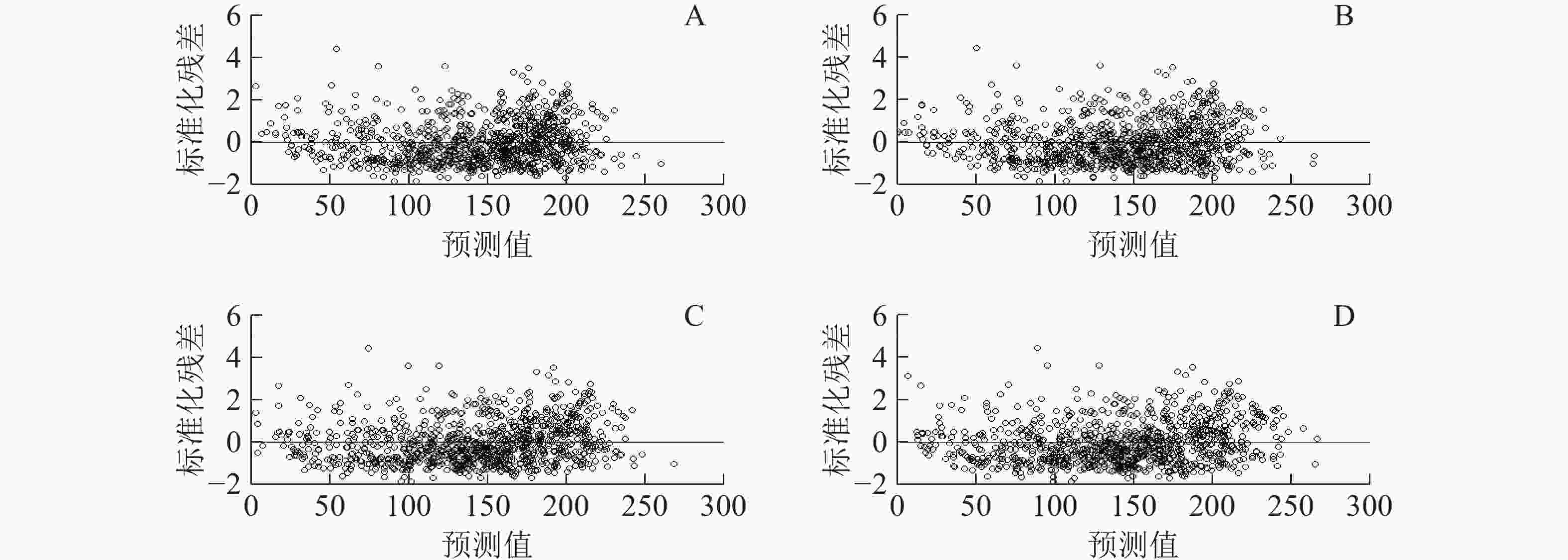
图 2 基于回归模型和混合效应模型生物量估测残差分布
Figure 2. Biomass estimation residual distribution based on regression model and mixed effect model
表 10 考虑组内协方差结构矩阵后各个效应混合模型比较结果
Table 10. Comparison results of mixed effects models considering intra-group covariance matrix
随机效应 协方差结构 AIC BIC logLik LRT P 区域效应 10 093.99 10 133.10 −5 038.993 指数函数 10 095.75 10 139.76 −5 038.877 0.233 1 0.629 0 高斯函数 10 095.99 10 139.99 −5 038.993 0.000 8 0.999 3 球面函数 10 093.70 10 137.71 −5 037.850 2.287 1 0.130 4 龄组效应 10 011.61 10 050.73 −4 997.806 指数函数 10 000.52 10 044.53 −4 991.262 13.088 0 <0.000 1 高斯函数 10 002.22 10 046.23 −4 992.110 0.040 2 0.841 0 球面函数 10 002.23 10 046.24 −4 992.117 11.378 0 0.000 7 两水平效应 9 956.50 10 010.29 −4 967.250 指数函数 9 956.43 10 015.10 −4 966.213 2.074 6 0.149 8 高斯函数 9 958.47 10 017.15 −4 967.237 0.027 3 0.870 1 球面函数 9 956.49 10 015.17 −4 966.248 2.003 7 0.156 9 通过以上步骤,确定了各水平最佳混合参数、组间矩阵结构和自相关矩阵结构后,把这几个方面综合考虑进行模拟,确定了各个效应混合模型形式。①区域效应混合模型:
$$ \left\{\begin{array}{l}{y}_{ij}=b-\left({a}_{1}+{a}_{1i}\right)A+{a}_{2}B+{a}_{3}C\\ {a}_{1i} \sim N(0,D)\end{array}\right.\text{。} $$ (11) ②龄组效应混合模型:
$$ \left\{\begin{split} & {y}_{ij}=b-\left({a}_{1}+{a}_{1ij}\right)A+{a}_{2}B+{a}_{3}C+{e}_{ij}\\ & {a}_{1ij} \sim N(0,D)\\ & {e}_{ij} \sim N\left(0,{\sigma }^{2}{R}_{i}\right),\;{R}_{i}={\sigma }_{i}^{2}\times {{\varGamma}} _{i}\left(\theta \right)\\ & {{\varGamma}} _{i}\left(\theta \right)=\exp\left(a{x}_{i}\right)\end{split}\right.\text{。} $$ (12) ③两水平混合效应模型:
$$ \left\{\begin{array}{l}{y}_{ij}=b-\left({a}_{1}+{a}_{1i}+{a}_{1ij}\right)A+{a}_{2}B+{a}_{3}C\\ {a}_{1i},\;{a}_{1ij} \sim N(0,{D}_{{\rm{UN}}})\end{array}\right.\text{。} $$ (13) 式(11)~(13)中:i为区域编号;j为龄组编号;a和b为常量;yij为i区域中j龄组云冷杉单位生物量预测值;A为B6波段值;B为B7波段值;C为NDVI值;a1、a2、a3分别为固定效应拟合参数;a1i、a1ij分别为区域效应和龄组效应随机参数;
$ {e}_{ij} $ 为模型误差项;$ {D}_{{\rm{UN}}} $ 为两水平组间方差-协方差矩阵;$ {R}_{i} $ 为组内方差-协方差结构;$ {\sigma }_{i}^{2} $ 为未知样地i的残差方差;${{\varGamma}} _{i}\left(\theta \right)$ 为龄组效应水平组内误差自相关结构矩阵;xi为自变量。 -
综合分析以上混合模型的拟合指标,得出各个效应水平上最优混合效应模型,其具体参数拟合结果如表11所示。结果表明:各个效应水平上的混合模型相较于回归模型均提高了其拟合精度。两水平混合效应模型的拟合指标优于单水平混合效应模型,而在单水平混合模型中,龄组效应混合模型的拟合指标优于区域效应混合模型。从模型的独立性检验结果上看(表11),各个效应水平上混合模型的总相对误差和平均相对误差均优于回归模型,而龄组效应混合模型有着最优的总相对误差和平均相对误差。
表 11 生物量混合效应模型拟合参数及独立性检验结果
Table 11. Biomass mixed effect model fitting parameters and independence test results
变量 区域效应混合模型 龄组效应混合模型 两水平混合效应模型 估计值 P 估计值 P 估计值 P 常量 278.430 <0.000 1 208.410 <0.000 1 220.590 <0.000 1 a1 −0.259 <0.000 1 −0.187 <0.000 1 −0.208 <0.000 1 a2 0.201 <0.000 1 0.143 <0.000 1 0.164 <0.000 1 a3 132.054 <0.000 1 107.874 <0.000 1 120.942 <0.000 1 残差 39.883 38.172 36.526 总相对误差 −4.564 −1.609 −7.539 平均相对误差 −0.462 −0.163 −0.765 说明:区域效应D矩阵(组间方差-协方差结构)为0.0010;龄组效应D矩阵为0.0007,R矩阵(组内方差-协方差结构)为0.465;两水平 D矩阵分别为0.0003和0.0002 -
由生物量分段残差检验结果(表12)可知:5种模型对云冷杉林生物量段的预估能力不同。总体来说,混合效应模型的预估能力优于回归模型和BP神经网络模型,5种模型均在150~200 t·hm−2生物量段预估能力最优,其绝对平均残差最小。在低生物量段(<100 t·hm−2),5种模型均出现了低值高估现象,但其两水平混合效应模型表现较优。在高生物量段(>233 t·hm−2),由于生物量值在生物量饱和阈值之上,5种模型均出现了严重的高值低估现象,但BP神经网络模型预估能力优于回归模型,而各效应水平混合模型均显著改善了高值低估,其平均残差由回归模型的79.39 t·hm−2、BP神经网络模型的72.37 t·hm−2降为区域效应混合模型的70.69 t·hm−2,龄组效应混合模型的68.65 t·hm−2,两水平混合效应模型的55.43 t·hm−2。
表 12 生物量分段残差检验
Table 12. Biomass segmentation residual test
生物量分段/(t·hm−2) 拟合模型 回归模型 BP神经网络模型 区域效应混合模型 龄组效应混合模型 两水平混合效应模型 0~50 −25.77 −26.39 −27.14 −25.34 −23.43 50~100 −15.35 −15.15 −13.87 −15.47 −14.85 100~150 −17.76 −10.69 −13.62 −12.63 −10.33 150~200 2.68 4.26 5.34 1.12 2.41 200~233 42.27 41.20 36.77 40.13 33.55 >233 79.39 72.37 70.69 68.65 55.43 -
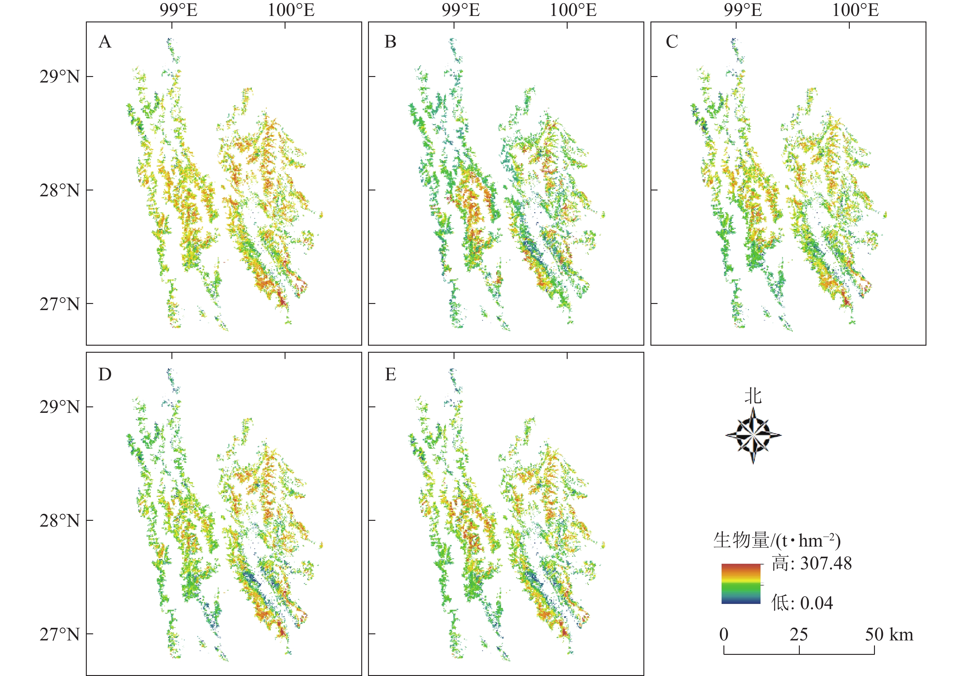
依据森林资源二类调查数据获取迪庆藏族自治州云冷杉林空间分布位置,基于Landsat 8 OLI影像,采用像元法,利用所构建模型计算每个小班像元内的云冷杉林生物量值,最终反演出整个研究区云冷杉林生物量(图3),其中回归模型(图3A)估算研究区云冷杉林地上生物量最大值为302.71 t·hm−2,最小值为0.38 t·hm−2,平均值为148.66 t·hm−2;BP神经网络模型(图3B)估算研究区云冷杉林地上生物量最大值为304.71 t·hm−2,最小值为0.19 t·hm−2,平均值为143.33 t·hm−2;区域效应混合模型(图3C)估算研究区云冷杉林地上生物量最大值为307.45 t·hm−2,最小值为0.10 t·hm−2,平均值为147.06 t·hm−2;龄组效应混合模型(图3D)估算研究区云冷杉林地上生物量,最大值为305.61 t·hm−2,最小值为0.25 t·hm−2,平均值为141.48 t·hm−2;两水平混合效应模型(图3E)估算研究区云冷杉林地上生物量最大值为302.43 t·hm−2,最小值为0.05 t·hm−2,平均值为141.63 t·hm−2。云冷杉林生物量的整体分布是沿着“三山”(怒山、云岭、中甸大雪山)纵向分布,符合云冷杉的生长习性。总体来说,各个效应水平的混合模型对云冷杉林生物量估测范围相较于回归模型及BP神经网络模型较宽,下限下移,上限上移,均值下移,在一定程度上能够解决生物量遥感估测中低值高估和高值低估问题。
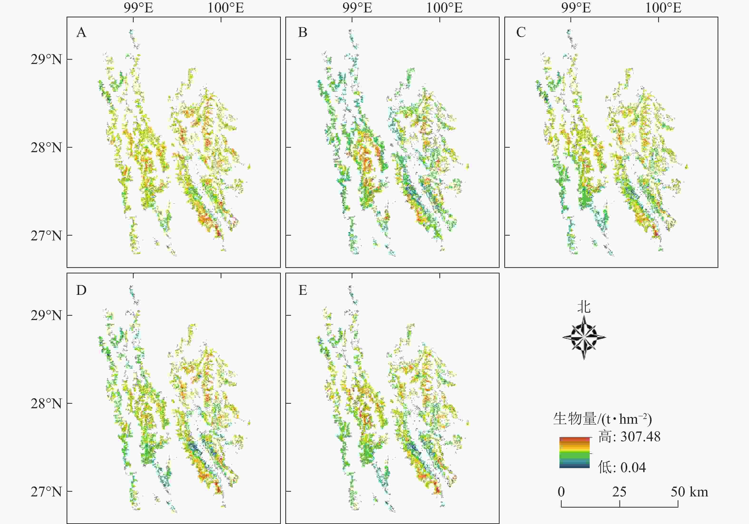
图 3 研究区云冷杉林地上生物量反演示意图
Figure 3. Biomass inversion of spruce-fir forests in the study area
-
本研究以小班尺度为研究单位,基于面状数据提取的遥感因子要比点状数据包含更多信息。一般小班地类划分最小面积为0.067 hm2进行森林资源调查,基于点状提取遥感因子反射率值不能够有效代表该小班实际遥感反射率,故本研究通过分区统计,优选出能够代表各小班内真实地物反射率信息统计值,反射率平均值与生物量相关性更强,符合统计学基本常识[26]。从云冷杉林生物量饱和值来看,本研究利用幂函数曲线拟合出的迪庆藏族自治州云冷杉林生物量饱和值高于赵盼盼[27]通过球状模型拟合的针叶林生物量饱和值。这是由于迪庆藏族自治州独特的地理位置,丰厚的水气条件,再加之云冷杉为当地优势树种,该地云冷杉林生物量均普遍高于其他地区。
由于缺乏足够多的样地信息,很少有研究能充分考虑林分间的异质性来构建生物量遥感估测模型,尤其是在高海拔、多山地的迪庆藏族自治州,不易开展外业工作,测树因子不易获取[17]。然而,本研究基于迪庆藏族自治州森林资源二类调查数据,有足够的样本信息针对云冷杉林林分间的异质性,完成生物量估测模型的构建;同时根据周律等[28]对于森林资源二类调查数据的可靠性验证结果,本研究构建了不同云冷杉林生物量遥感估测模型,探索提高生物量估测精度的方法。从最终拟合模型的精度评价与检验结果看,各个效应水平的混合模型的拟合精度均优于回归模型,且独立性检验指标总相对误差和平均相对误差也均优于回归模型和BP神经网络模型。这也在生物量分段误差检验结果中有所表现,混合效应模型在一定程度上降低了回归模型和BP神经网络模型估测生物量普遍存在的低值高估和高值低估现象,尤其是在饱和阈值之后生物量的估测误差。这是因为混合效应模型能够针对不同效应水平分组数据分别构建预估模型。这类似于利用分层思想,在充分考虑林分间的异质性下,提高模型的拟合和预估能力。这与李春明[22]、符利勇等[23]对混合效应模型研究结果一致。
-
基于面状数据提取遥感因子信息平均值能够有效代表真实地物遥感因子反射率信息,与生物量相关性更高;以Landsat 8 OLI B6波段采用幂函数拟合出迪庆藏族自治州云冷杉林生物量饱和值为233 t·hm−2。
充分考虑林分间异质性各效应水平的混合模型均提高了回归模型的拟合精度,独立性检验指标均优于回归模型和BP神经网络模型,其各个生物量分段平均残差也均有所降低,更大的估测范围显著降低了一般模型生物量遥感估测的低值高估尤其饱和阈值之后高值低估的影响,提高了预估精度。
Remote sensing estimation of aboveground biomass of spruce-fir forests in Diqing based on mixed effect models
-
摘要:
目的 确定云冷杉林生物量光学遥感估测饱和值,探索提高生物量遥感估测精度。 方法 以云南省迪庆藏族自治州云冷杉林为研究对象,根据森林资源二类调查数据,结合同时期Landsat 8 OLI遥感影像,利用随机选取的小班样本数据提取遥感因子反射率统计值,并与生物量进行曲线拟合,求解云冷杉林生物量饱和值,建立云冷杉生物量回归估测模型、BP神经网络模型。同时基于回归模型构建考虑区域、龄组效应的单水平和嵌套两水平(区域+龄组)混合效应模型,反演研究区云冷杉林地上生物量。 结果 利用幂函数拟合得到迪庆藏族自治州云冷杉林生物量饱和值为233 t·hm−2;最优回归估测模型调整决定系数(Ra2)为0.606,高于BP神经网络模型的Ra2(0.542),各个效应水平混合模型的拟合精度与独立性检验指标均优于回归模型。考虑两水平的混合效应模型有最优的拟合精度,而考虑龄组效应水平的混合模型有最优的独立性检验指标。混合效应模型在低生物量段(<100 t·hm−2)和高生物量段(>233 t·hm−2)均显著降低了回归模型和BP神经网络模型的估测平均残差。 结论 混合效应模型有更宽的估测范围,在一定程度上减小低值高估与数据饱和造成的高值低估影响,提高了预估精度。图3表12参28 Abstract:Objective The objective of this study is to determine the saturation value of optical remote sensing estimation of spruce-fir forest biomass, and to improve the accuracy of remote sensing estimation of biomass. Method Taking the spruce-fir forests in Diqing Tibetan Autonomous Prefecture as the research object, the saturation value of the spruce-fir biomass was calculated by curve fitting, Tibetan Autonomous and the regression estimation model and BP neural network model of the spruce-fir biomass were established using the forest management inventory (FMI) data combined with Landsat 8 OLI remote sensing image in the contract period and the statistical value of remote sensing factor reflectance extracted from the randomly selected small class sample data. At the same time, based on the regression model, single level and nested two-level(region+age group)mixed effect models considering regional and age group effects were constructed to estimate the aboveground biomass of spruce-fir forests in the study area. Result The biomass saturation value of the spruce-fir forests in Diqing Tibetan Autonomous Prefecture was 233 t·hm−2 by power function fitting. The adjusted determination coefficient of the optimal regression estimation model $R_{\rm{a}}^{2}$ was 0.606, which was higher than$R_{\rm{a}}^{2}$ (0.542) of the BP neural network model. The fitting accuracy and independence test indexes of the mixed model of each effect level were better than those of the regression model. The two-level mixed effect model had the best fitting accuracy, while the mixed model with age group effect level had the best independence test index. The mixed effect model significantly reduced the average residual error of regression model and BP neural network model in the low biomass section (<100 t·hm−2), especially in the high biomass section (>233 t·hm−2).Conclusion The mixed effect model has a wider estimation range, which can reduce the impact of low overestimation and high underestimation caused by data saturation, and improve prediction accuracy. [Ch, 3 fig. 12 tab. 28 ref.] -
图 1 幂函数拟合云冷杉林生物量饱和曲线
Figure 1 Power function fitting curve of spruce-fir forest biomass saturation
图 2 基于回归模型和混合效应模型生物量估测残差分布
A. 基本模型;B. 区域效应混合模型;C. 龄组效应混合模型;D. 两水平混合效应模型
Figure 2 Biomass estimation residual distribution based on regression model and mixed effect model
图 3 研究区云冷杉林地上生物量反演示意图
A. 回归模型;B. BP神经网络模型;C. 区域效应混合模型;D. 龄组效应混合模型;E. 两水平混合效应模型
Figure 3 Biomass inversion of spruce-fir forests in the study area
表 1 研究区Landsat 8 OLI影像基本信息
Table 1. Basic information of Landsat 8 OLI images in study area
影像ID 获取时间 条带号 太阳方位角/(°) 太阳高度角/(°) 平均云量/% LC81310412016341LGN00 2016-12-06 131/041 156.524 36.313 1.04 LC81320402016348LGN00 2016-12-13 132/040 156.677 34.220 0.73 LC81320412016348LGN00 2016-12-13 132/041 156.001 35.443 0.76  下载: 导出CSV
表 2 云冷杉蓄积量—生物量转换因子信息指数
Table 2. Spruce and fir storage—biomass conversion factor information index
树种 模型公式 FBE DSV 幼龄林 中龄林 近熟林 成熟林 过熟林 乔木层 云杉 MA=VFBEDSV 2.326 5 1.516 4 1.473 0 1.427 4 1.264 2 0.342 冷杉 1.327 9 1.339 3 1.333 6 1.309 7 1.285 9 0.366 说明:MA为单位面积生物量;V为单位面积蓄积量;FBE为蓄积生物量转换系数;DSV为木材基本密度
下载: 导出CSV
表 3 建模及检验数据基本情况
Table 3. Modeling and testing data
统计量 建模/训练数据(n=983) 检验数据(n=245) 单位面积蓄
积量/(m3∙hm−2)单位面积生
物量/(t∙hm−2)单位面积蓄
积量/(m3∙hm−2)单位面积生
物量/(t∙hm−2)最小值 8.33 5.74 28.57 14.37 最大值 651.82 314.83 598.92 287.88 平均值 294.73 141.66 298.78 143.57 标准差 137.54 65.43 122.51 58.65
下载: 导出CSV
表 5 生物量与遥感因子各统计值相关性
Table 5. Significant Pearson correlation coefficients between remote sensing factors and AGB
遥感因子 MEAN MAX MIN 遥感因子 MEAN MAX MIN ALBEDO −0.555** −0.065* −0.449** ND67 0.439** 0.160** 0.317** ARVI 0.469** 0.251** 0.193** NDVI 0.329** 0.216** 0.069* B −0.540** −0.055 −0.430** NLI 0.165** 0.207** 0.091** B1 −0.168** 0.010 −0.092** PC1-A −0.682** −0.154** 0.323** B2 −0.187** 0.008 −0.097** PC1-B −0.711** −0.165** 0.337** B3 −0.238** 0.001 −0.095** PC1-P 0.616** 0.383** −0.180** B4 −0.334** −0.018 −0.096** PC2-A 0.440** 0.172** −0.110** B5 −0.296** 0.003 −0.100** PC2-B 0.099** 0.040 −0.097** B6 −0.762** −0.333** −0.101** PC2-P 0.670** 0.349** 0.085** B7 −0.705** −0.345** −0.219** PC3-A −0.094** 0.016 −0.004 DVI −0.050 0.036 −0.220** PC3-B −0.039 0.049 −0.470** G 0.057 0.051 −0.203** PC3-P −0.197** 0.006 −0.531** KT1 −0.555** −0.060* −0.203** PVI −0.237** 0.004 0.163** KT2 0.070* 0.053 −0.521** RVI 0.102** −0.002 0.325** KT3 0.534** 0.126** −0.523** SARV −0.036 −0.041 0.176** MSAVI 0.326** 0.215** −0.430** SAV12 0.326** 0.215** 0.361** MSR 0.269** 0.009 −0.430** SAVI 0.329** 0.216** 0.043 MVI5 0.626** 0.436** −0.057* SR 0.102** −0.002 −0.016 MVI7 0.619** 0.363** −0.018 TVI 0.329** 0.217** −0.052 ND43 −0.490** −0.251** −0.441** W 0.497** 0.114** −0.174** ND563 −0.075* 0.010 −0.015 说明:**表示极显著相关(P<0.01);*表示显著相关(P<0.05)
下载: 导出CSV
表 6 基于不同曲线拟合饱和值结果
Table 6. Results of fitting saturation values based on different curves
函数 R2 P 对数函数 0.555 0.000 二次项函数 0.583 0.000 三次项函数 0.584 0.000 幂函数 0.590 0.000
下载: 导出CSV
表 7 基于单水平混合参数选择拟合结果
Table 7. Selection of fitting results based on single-level mixing parameters
模型 混合参数 区域效应 龄组效应 AIC BIC logLik AIC BIC logLik 基础模型 无 10 129.57 10 154.04 −5 059.787 10 129.57 10 154.04 −5 059.787 模型1 a1 10 093.99 10 133.10 −5 038.993 10 011.61 10 050.73 −4 997.806 模型2 a2 10 102.12 10 141.24 −5 043.062 10 016.07 10 055.18 −5 000.034 模型3 a3 不收敛 10 023.89 10 063.00 −5 003.943 模型4 a1, a2 10 099.99 10 153.78 −5 038.996 10 017.62 10 071.41 −4 997.812 模型5 a1, a3 10 100.01 10 153.80 −5 039.007 10 017.66 10 071.44 −4 997.829 模型6 a2, a3 10 108.13 10 161.92 −5 043.066 10 022.21 10 075.99 −5 000.105 模型7 a1, a2, a3 10 108.00 10 181.34 −5 038.998 10 023.67 10 053.00 −5 005.834
下载: 导出CSV
表 8 基于两水平混合参数选择拟合结果
Table 8. Selection of fitting results based on two levels of mixing parameters
模型 区域效应 龄组效应 AIC BIC logLik a1 a2 a3 a1 a2 a3 模型1 √ √ 9 956.50 10 010.29 −4 967.250 模型2 √ √ √ 9 958.93 10 012.71 −4 968.464 模型3 √ √ √ √ 9 957.83 10 045.84 −4 960.915 模型4 √ √ √ √ √ 9 963.75 10 066.43 −4 960.872 模型5 √ √ √ √ √ √ 9 971.72 10 093.96 −4 960.862 说明:带√的变量表示模型包含这个随机参数
下载: 导出CSV
表 9 基于随机参数不同组间方差-协方差结构混合模型拟合结果
Table 9. Mixed model fitting results of variance-covariance structure between groups based on random parameters
方差-协方差结构 自由度 AIC BIC logLik 似然比检验(LRT) P 广义正定矩阵(UN) 11 9 956.50 10 010.29 −4 967.250 复合对称(CS) 10 9 958.34 10 012.24 −4 969.170 18.396 56 <0.000 1 对角矩阵(UN1) 9 9 965.69 10 009.70 −4 973.846 13.190 81 0.001 4
下载: 导出CSV
表 10 考虑组内协方差结构矩阵后各个效应混合模型比较结果
Table 10. Comparison results of mixed effects models considering intra-group covariance matrix
随机效应 协方差结构 AIC BIC logLik LRT P 区域效应 10 093.99 10 133.10 −5 038.993 指数函数 10 095.75 10 139.76 −5 038.877 0.233 1 0.629 0 高斯函数 10 095.99 10 139.99 −5 038.993 0.000 8 0.999 3 球面函数 10 093.70 10 137.71 −5 037.850 2.287 1 0.130 4 龄组效应 10 011.61 10 050.73 −4 997.806 指数函数 10 000.52 10 044.53 −4 991.262 13.088 0 <0.000 1 高斯函数 10 002.22 10 046.23 −4 992.110 0.040 2 0.841 0 球面函数 10 002.23 10 046.24 −4 992.117 11.378 0 0.000 7 两水平效应 9 956.50 10 010.29 −4 967.250 指数函数 9 956.43 10 015.10 −4 966.213 2.074 6 0.149 8 高斯函数 9 958.47 10 017.15 −4 967.237 0.027 3 0.870 1 球面函数 9 956.49 10 015.17 −4 966.248 2.003 7 0.156 9
下载: 导出CSV
表 11 生物量混合效应模型拟合参数及独立性检验结果
Table 11. Biomass mixed effect model fitting parameters and independence test results
变量 区域效应混合模型 龄组效应混合模型 两水平混合效应模型 估计值 P 估计值 P 估计值 P 常量 278.430 <0.000 1 208.410 <0.000 1 220.590 <0.000 1 a1 −0.259 <0.000 1 −0.187 <0.000 1 −0.208 <0.000 1 a2 0.201 <0.000 1 0.143 <0.000 1 0.164 <0.000 1 a3 132.054 <0.000 1 107.874 <0.000 1 120.942 <0.000 1 残差 39.883 38.172 36.526 总相对误差 −4.564 −1.609 −7.539 平均相对误差 −0.462 −0.163 −0.765 说明:区域效应D矩阵(组间方差-协方差结构)为0.0010;龄组效应D矩阵为0.0007,R矩阵(组内方差-协方差结构)为0.465;两水平 D矩阵分别为0.0003和0.0002
下载: 导出CSV
表 12 生物量分段残差检验
Table 12. Biomass segmentation residual test
生物量分段/(t·hm−2) 拟合模型 回归模型 BP神经网络模型 区域效应混合模型 龄组效应混合模型 两水平混合效应模型 0~50 −25.77 −26.39 −27.14 −25.34 −23.43 50~100 −15.35 −15.15 −13.87 −15.47 −14.85 100~150 −17.76 −10.69 −13.62 −12.63 −10.33 150~200 2.68 4.26 5.34 1.12 2.41 200~233 42.27 41.20 36.77 40.13 33.55 >233 79.39 72.37 70.69 68.65 55.43
下载: 导出CSV
-
[1] 魏殿生. 造林绿化与气候变化-碳汇问题研究[M]. 北京: 中国林业出版社, 2003. [2] 刘茜, 杨乐, 柳钦火, 等. 森林地上生物量遥感反演方法综述[J]. 遥感学报, 2015, 19(1): 62 − 74. LIU Qian, YANG Le, LIU Qinhuo, et al. Review of forest above ground biomass inversion methods based on remote sensing technology [J]. J Remote Sensing, 2015, 19(1): 62 − 74. [3] 于艳梅, 徐俊增, 彭世彰, 等. 不同水分条件下水稻光合作用的光响应模型的比较[J]. 节水灌溉, 2012(10): 30 − 33. YU Yanmei, XU Junzeng, PENG Shizhang, et al. Evaluation of photosynthesis light response model for rice leaf under different water conditions [J]. Water Sav Irrig, 2012(10): 30 − 33. [4] XIE Yichun, SHA Zongyao, YU Mei, et al. A comparison of two models with Landsat data for estimating above ground grassland biomass in Inner Mongolia, China [J]. Ecol Modelling, 2009, 220(15): 1810 − 1818. [5] POWELL S L, COHEN W B, HEALEY S P, et al. Quantification of live aboveground forest biomass dynamics with Landsat time-series and field inventory data: a comparison of empirical modeling approaches [J]. Remote Sensing Environ, 2010, 114(5): 1053 − 1068. [6] 国庆喜, 张锋. 基于遥感信息估测森林的生物量[J]. 东北林业大学学报, 2003, 31(2): 13 − 16. GUO Qingxi, ZHANG Feng. Estimation of forest biomass based on remote sensing [J]. J Northeast For Univ, 2003, 31(2): 13 − 16. [7] 欧光龙, 胥辉, 王俊峰, 等. 思茅松天然林林分生物量混合效应模型构建[J]. 北京林业大学学报, 2015, 37(3): 101 − 110. OU Guanglong, XU Hui, WANG Junfeng, et al. Building mixed effect models of stand biomass for Simao pine(Pinus kesiya var. langbianensis) natural forest [J]. J Beijing For Univ, 2015, 37(3): 101 − 110. [8] 姜立春, 李凤日. 混合效应模型在林业建模中的应用[M]. 北京: 科学出版社, 2014. [9] 曾伟生, 唐守正, 夏忠胜, 等. 利用线性混合模型和哑变量模型方法建立贵州省通用性生物量方程[J]. 林业科学研究, 2011, 24(3): 285 − 291. ZENG Weisheng, TANG Shouzheng, XIA Zhongsheng, et al. Using linear mixed model and dummy variable model approaches to construct generalized single-tree biomass equations in Guizhou [J]. For Res, 2011, 24(3): 285 − 291. [10] 董利虎, 李凤日, 贾炜玮. 基于线性混合效应的红松人工林枝条生物量模型[J]. 应用生态学报, 2013, 24(12): 3391 − 3398. DONG Lihu, LI Fengri, JIA Weiwei. Linear mixed modeling of branch biomass for Korean pine plantation [J]. Chin J Appl Ecol, 2013, 24(12): 3391 − 3398. [11] 胥喆, 舒清态, 杨凯博, 等. 基于非线性混合效应的高山松林生物量模型研究[J]. 江西农业大学学报, 2017, 39(1): 101 − 110. XU Zhe, SHU Qingtai, YANG Kaibo, et al. A study on biomass model of Pinus densata forest based on nonlinear mixed effects [J]. Acta Agric Univ Jiangxi, 2017, 39(1): 101 − 110. [12] 胥辉, 张子翼, 欧光龙, 等. 云南省森林生物量和碳储量估算及分布研究[M]. 昆明: 云南科技出版社, 2019. [13] 周小成, 庄海东, 陈铭潮, 等. 面向小班对象的森林资源变化遥感监测方法: 以福建省厦门市为例[J]. 资源科学, 2013, 35(8): 1710 − 1718. ZHOU Xiaocheng, ZHUANG Haidong, CHEN Mingchao, et al. A method to extract forest cover change by object-oriented classification [J]. Resour Sci, 2013, 35(8): 1710 − 1718. [14] MOZGERIS G. Estimation and use of continuous surfaces of forest parameters: options for lithuanian forest inventory [J]. Baltic For, 2008, 14(2): 176 − 184. [15] FERNÁNDEZ-MANSO O, FERNÁNDEZ-MANSO A, QUINTANO C. Estimation of aboveground biomass in Mediterranean forests by statistical modelling of ASTER fraction images [J]. Int J Appl Earth Obs Geoinf, 2014, 31(31): 45 − 56. [16] 郎晓雪, 许彦红, 舒清态, 等. 香格里拉市云冷杉林蓄积量遥感估测非参数模型研究[J]. 西南林业大学学报, 2019, 39(1): 146 − 151. LANG Xiaoxue, XU Yanhong, SHU Qingtai, et al. Nonparametric model for remote sensing estimating the volume of spruce-fir forest in Shangri-La [J]. J Southwest For Univ, 2019, 39(1): 146 − 151. [17] 陆驰, 张加龙, 王爱芸, 等. 基于森林小班的香格里拉市高山松生物量遥感建模[J]. 西南林业大学学报, 2017, 37(3): 158 − 164. LU Chi, ZHANG Jialong, WANG Aiyun, et al. Building the model on the estimation of Pinus densata’s biomass in Shangri-La City based on forest subcompartment and remote sensing images [J]. J Southwest For Univ, 2017, 37(3): 158 − 164. [18] 董宇. 基于遥感信息估测将乐县森林生物量的研究[D]. 北京: 北京林业大学, 2012. DONG Yu. Estimate Forest Biomass in Jiangle based on Remote Sensing[D]. Beijing: Beijing Forestry University, 2012. [19] 孙雪莲. 基于Landsat 8-OLI的香格里拉高山松林生物量遥感估测模型研究[D]. 昆明: 西南林业大学, 2016. SUN Xuelian. Biomass Estimation Model of Pinus densata Forests in Shangri-La City based on Landsat 8-OLI by Remote Sensing[D]. Kunming: Southwest Forestry University, 2016. [20] 岳彩荣. 香格里拉县森林生物量遥感估测研究[D]. 北京: 北京林业大学, 2012. YUE Cairong. Forest Biomass Estimation in Shangri-La County based on Remote Sensing[D]. Beijing: Beijing Forestry University, 2012. [21] 邱布布, 徐丽华, 张茂震, 等. 基于Landsat OLI和ETM+的杭州城市绿地地上生物量估算比较研究[J]. 西北林学院学报, 2018, 33(1): 225 − 232. QIU Bubu, XU Lihua, ZHANG Maozhen, et al. Estimation of above-ground biomass of urban green land in Hangzhou based on Landsat OLI and ETM+ data [J]. J Northwest For Univ, 2018, 33(1): 225 − 232. [22] 李春明. 基于两层次线性混合效应模型的杉木林单木胸径生长量模型[J]. 林业科学, 2012, 48(3): 66 − 73. LI Chunming. Individual tree diameter increment model for Chinese fir plantation based on two-level linear mixed effects models [J]. Sci Silv Sin, 2012, 48(3): 66 − 73. [23] 符利勇, 李永慈, 李春明, 等. 利用2种非线性混合效应模型(2水平)对杉木林胸径生长量的分析[J]. 林业科学, 2012, 48(5): 36 − 43. FU Liyong, LI Yongci, LI Chunming, et al. Analysis of the basal area for Chinese fir plantation using two kinds of nonlinear mixed effects model(two levels) [J]. Sci Silv Sin, 2012, 48(5): 36 − 43. [24] PINHEIRO J C, BATES D M. Mixed Effects Models in S and S-Plus[M]. New York: Springer Verlag, 2000. [25] VONESH E F, CHINCHILLI V M. Linear and Nonlinear Models for the Analysis of Repeated Measurements[M]. New York: Marcel Dekker Inc, 1997. [26] 王磊, 徐晓岭. 统计学[M]. 北京: 人民邮电出版社, 2015. [27] 赵盼盼. 基于Landsat TM和ALOS PALSAR数据的森林地上生物量估测研究[D]. 杭州: 浙江农林大学, 2016. ZHAO Panpan. Aboveground Forest Biomass Estimation based on Landsat TM and ALOS PALSAR Data[D]. Hangzhou: Zhejiang A&F University, 2016. [28] 周律, 欧光龙, 王俊峰, 等. 基于空间回归模型的思茅松林生物量遥感估测及光饱和点确定[J]. 林业科学, 2020, 56(3): 38 − 47. ZHOU Lü, OU Guanglong, WANG Junfeng, et al. Light saturation point determination and biomass remote sensing estimation of Pinus kesiya var. langbianensis forest based on spatial regression models [J]. Sci Silv Sin, 2020, 56(3): 38 − 47. -

-
链接本文:
https://zlxb.zafu.edu.cn/article/doi/10.11833/j.issn.2095-0756.20200327
 点击查看大图

计量
- 文章访问数: 2410
- HTML全文浏览量: 641
- PDF下载量: 72
- 被引次数: 0


